Download
1 / 41
560 likes | 886 Views
2006 Speech/Audio Signal Processing in MATLAB/Simulink. Speech/Audio Signal Processing in MATLAB/Simulink. J.-S. Roger Jang ( 張智星 ) CS Dept, Tsing-Hua Univ, Taiwan ( 清華大學 資訊系 ) http://www.cs.nthu.edu.tw/~jang jang@cs.nthu.edu.tw. Outline. Wave file manipulation

E N D
2006 Speech/Audio Signal Processing in MATLAB/Simulink Speech/Audio Signal Processing in MATLAB/Simulink • J.-S. Roger Jang (張智星) • CS Dept, Tsing-Hua Univ, Taiwan • (清華大學 資訊系) • http://www.cs.nthu.edu.tw/~jang • jang@cs.nthu.edu.tw
Outline • Wave file manipulation Reading, writing, recording ... • Time-domain processing Delay, filtering, sptools … • Frequency-domain processing Spectrogram • Pitch determination Auto-correlation, SIFT, AMDF, HPS ... • Others Formant estimation, speech coding
Toolbox/Blockset Used • MATLAB • Simulink • Signal Processing Toolbox • DSP Blockset
MATLAB Primer • Before you start, you need to get familiar with MATLAB. Please read “MATLAB Primer” at the following page: • http://neural.cs.nthu.edu.tw/jang/demo/demoDownload.asp • Exercise: • Please plot two curves y=sin(2*t) and y=cos(3*t) in the same figure. • Please plot x vs. y where x=sin(2*t) and y=cos(3*t).
To Read a Wave File • To read a MS .wav file (PCM format only): wavread y = wavread(file) […] = wavread(file, [n1, n2]) [y, fs, nbits, opts] = wavread(file) […] = wavread(file, n) [y, fs, nbits] = wavread(file) • If the wav file is stereo, y will be a two-column matrix.
To Read a Wav File • Example (wavRead01.m): [y, fs] = wavread('singapore.wav'); plot((1:length(y))/fs, y); xlabel('Time in seconds'); ylabel('Amplitude'); • Exercise: • Plot the waveform of “rrrrr.wav”. Use MATLAB’s “zoom” button to find the consecutive curling “R” occurs. • Plot the two-channel waveform in “flanger.wav”.
wavRead02.m: [y, fs] = wavread(‘flanger.wav’); subplot(2,1,1), plot((1:length(y))/fs, y(:,1)); subplot(2,1,2), plot((1:length(y))/fs, y(:,2)); Solution to the Previous Exercise
To Play Wav Files • To play sound using Windows audio output device: wavplay, sound, soundsc wavplay(y, fs) wavplay(y, fs, ‘async’): non-blocking call wavplay(y, fs, ‘sync’): blocking call sound(y, fs) soundsc(…): autoscale the sound • Example (wavPlay01.m): [y, fs] = wavread(‘rrrrr.wav’); wavplay(y, fs); • Exercise: Follow the example to play “flanger.wav”.
To Read/Play Using DSP Blocks • To read/play sound using DSP Blockset: DSP Blockset/DSP Sources/From Wave File DSP Blockset/DSP Sinks/To Wave Device • Example: • Exercise: Create a model as shown above. Frame-based operation!
Solution • Solution to the previous exercise: • slWavFilePlay01.mdl
To Write a Wave File • To write MS wave files: wavwrite wavwrite(y, fs, nbits, wavefile) “nbits” must be 8 or 16. “y” must have two columns for stereo data. Amplitude values outside [-1,1] are clipped. • Example (wavWrite01.m): [y, fs] = wavread(‘rrrrr.wav’); wavwrite(y, fs*1.2, 8, ‘testout.wav’); !start testout.wav • Exercise: Try out the above example.
To Record a Wave File • To record wave files: 1. Use the recording utility under WinXP. 2. Use “wavrecord” under MATLAB. 3. Use “From Wave Device” under Simulink, under “DSP Blocksets/Platform Specific IO/Windows (Win32)” • Example: 1. Go ahead and try WinXP recording utility! 2. Try “wavRecord01.m” 3. Try “slWavFileRecord01.mdl” • Exercise: Try out the above examples.
Time-Domain Speech Signals • A typical time-domain plot of speech signals: Amplitude: volume or intensity Frequency: pitch
Changing Wave Playback Param. • To control the play of a sound: • Normal: wavplay(y, fs) • High volume: wavplay(2*y, fs) • Low volume: wavplay(0.5*y, fs) • High pitch (and faster): wavplay(y, 1.2*fs) • Low pitch (and slower): wavplay(y, 0.8*fs) • Exercise: • Try “wavPlay01.m” and trace the code. • Create “wavPlay02.m” such that you can record your own voice on the fly.
Time-Domain Signal Processing • Take-home exrecise: How to get a high pitch with the same time span?
Synthetic Sounds • Use a sine wave generator (under DSP blocksets) to produce sounds Single frequency: Multiple frequencies: Amplitude modulation: • Exercise: Create the above models.
Solution • Solution to the previous exercise: • sineSource01 • sineSource02 • sineSource03
Delay in Speech/Audio • What is a delay in a signal? y(n) --> y(n-k) • What effects can delay generate? Echo Reverberation Chorus Flanging
-k z Single Delay in Audio Signal • Block diagram: Input a Output u(n) y(n) = u(n) + a*u(n-k) • Simulink model: • Exercise: Create the above model.
-k z Multiple Delay in Audio Signal • How to create “karaoke” effects: a Input Output y(n) u(n) 2 3 y(n) = u(n) + a u(n-k) + a u(n-2k) + a u(n-3k) ... • Simulink model:
Multiple Delay in Audio Signal • Parameter values: • Feedback gain a < 1 • Actual delay time = k/fs • Exercise: • Create the above model and change some parameters to see their effects. • Modify the model to take microphone input (so you can start singing karaoke now!) • Use a “configurable subsystem” to include all possible input files and the microphone. (See next page.)
Multiple Delay in Audio Signal • How to use “configurable subsystem” block? 1. Create a library (say, wavinput.mdl) 2. Get a block of “configurable subsystem” 3. Fill the dialog box with the library name
Audio Flanging • Flanging sound: • A sound similar to the sound of a jet plane flying overhead, or a "whooshing" sound • “Pitch modulation” due to a variable delay • Simulink demo: • dspafxf.mdl (all platforms) • dspafxf_nt.mdl (for 95/98/NT)
Audio Flanging • Simulink model: Original spectrogram: Modified spectrogram:
Signal Processing Using sptool • To invoke sptool, type “sptool”.
Speech Production • How is speech produced? Speech is produced when air is forced from the lungs through the vocal cords (glottis) and along the vocal tract. • Analogy to System Theory: Input: air forced into the vocal cords Output: media vibration System (or filter): vocal tract Pitch frequency: frequency of the input Formant frequency: resonant frequency
Source Filter Model of Speech • The source-filter model of speech production: Speech is split into a rapidly varying excitation signal and a slowly varying filter. The envelope of the power spectra contains the vocal tract information. Two important characteristics of the model are fundamental (pitch) frequency (f0) and formants (F1, F2, F3, …)
Frame Analysis of Speech Signal Speech wave form : Zoom in Overlap Frame
Spectrogram • Spectrogram (specgram.m) displays short-time frequency contents: Wave form : Spectrogram :
Real-time Spectrogram • Try “dspstfft_win32”: Spectrum: Spectrogram:
Pitch and Formants • Pitch and formants can be defined visually: Pitch period = 1/f0 First formant F1 Second formant F2
Spectrogram Reading • Spectrogram Reading • http://cslu.cse.ogi.edu/tutordemos/SpectrogramReading/spectrogram_reading.html Waveform: Spectrogram: “compute”
Pitch Determination Algorithms • Time-domain: • Auto-correlation • AMDF (Average Magnitude Difference Function) • Gold-Rabiner algorithm (1969) • Frequency-domain: • Cepstrum (Noll 1964) • Harmonic product spectrum (Schroeder 1968) • Others: • SIFT (Simple inverse filter tracking) • Maximum likelihood • Neural network approach
Autocorrelation of Each Frame • Let s(k) be a frame of size 128. 1 128 s(k): s(k-h): h=30 x(30) = dot prod. of overlapped = sum(s(31:128).*s(1:99) Autocorrelation x(h): Pitch period 30
Autocorrelation via DSP Blockset • Real-time autocorrelation demo: • Exercise: Construct the above model and try it.
Pitch Tracking via Autocorrelation • Real-time pitch tracking via autocorrelation: pitch2.mdl
Formant Analysis • Characteristics of formants: • Formants are perceptually defined. • The corresponding physical property is the frequencies of resonances of the vocal tract. • Formant analysis is useful as the position of the first two formants pretty much identifies a vowel. • Computation methods: • Peak picking on the smoothed spectrum • Peak picking on the LP spectrum • Factoring for the LP roots • Fitting of mixture of Gaussians
Formant Analysis • Track Draw: • A package for formant synthesis with options to sketch formant tracks on a spectrogram. • http://www.utdallas.edu/~assmann/TRACKDRAW/trackdraw.html • Formant Location Algorithm • MATLAB code by Michelle Jamrozik • http://ece.clemson.edu/speech/files.htm
Speech Waveform Coding • Time domain coding • PCM: Pulse Code Modulation • DPCM: Differential PCM • ADPCM: Adaptive Differential PCM (dspadpcm.mdl) • Frequency domain coding • Sub-band coding • Transform coding • Speech Coding in MATLAB http://www.eas.asu.edu/~speech/education/educ1.html
Conclusions • Ideal tools for speech/audio signal processing: • MATLAB • Simulink • Signal Processing Toolbox • DSP Blockset • Advantages: • Reliable functions: well-established and tested • Visible graphical algorithm design tools • High-level programming language yet C-compatible • Powerful visualization capabilities • Easy debugging • Integrated environment
References [1] “Discrete-Time Processing of Speech Signals”, by Deller, Proakis and Hansen, Prentice Hall, 1993 [2] “Fundamentals of Speech Recognition”, by Rabiner and Juang, Prentice Hall, 1993 [3] “Effects Explained”, http://www.harmony-central.com/Effects/effects-explained.html [4] “TrackDraw”, http://www.utdallas.edu/~assmann/TRACKDRAW/trackdraw.html [5] “Speech Coding in MATLAB”, http://www.eas.asu.edu/~speech/education/educ1.html