Download

1 / 65
650 likes | 819 Views
The Need For Resampling In Multiple testing. Correlation Structures. Tukey’s T Method exploit the correlation structure between the test statistics, and have somewhat smaller critical value than the Bonferroni-style critical values.

E N D
Correlation Structures • Tukey’s T Method exploit the correlation structure between the test statistics, and have somewhat smaller critical value than the Bonferroni-style critical values. • It is easier to obtain a statistically significant result when correlation structures are incorporated.
Correlation Structures • The incorporation of correlation structure results in a smaller adjusted p-value than Bonferroni-style adjustment, again resulting in more powerful tests. • The incorporation of correlation structures can be very important when the correlations are extremely large.
Correlation Structures • Often, certain variables are recognized as duplicating information and are dropped, or perhaps the variables are combined into a single measure. • In the case, the correlations among the resulting variables is less extreme.
Correlation Structures • In cases of moderate correlation structures, the distribution between the Bonferroni adjustment and the exact adjustment can be very slight. • Bonferroni inequality: Pr{∩1r Ai} ≧1-Σ1r Pr{Aic} A small value of ‘’Pr{Aic}’’corresponds to a small per-comparison error rate.
Correlation Structures • The incorporating dependence structure becomes less important for smaller significant levels. • If a Bonferroni-style correction is reasonable, then why bother with resampling?
Distributional Characteristics • Other distributional characteristics, such as discreteness and skewness, can have dramatic effect, even for small p-value. • The nonnormality is of equal or greater concern than correlation structure in multiple testing application.
The Need For Resampling In Multiple testing Distribution Of Extremal Statistics Under Nonnormality
Noreen’s analysis of tests for a single lognormal mean • Yij are observations. i=1,..,10, j=1,..,n • All observations are independent and identically distributed as ez, where Z denotes a standard normal random variable. • The hypotheses tested are Hi: E(Yij)=√e, with upper or lower-tailed alternatives. • t=(y-√e)/(s/√n) _
Distributions of t-statistics • For each graph there were 40000 t-statistics, all simulated using lognormal yij. • The solid lines (actual) show the distribution of t when sampling from lognormal population, and the dotted lines (nominal) show the distribution of t when sampling from normal population.
Distributions of t-statistics • The lower tail area of the actual distribution of t-statistic is larger than the corresponding tail of the approximating Student’s t-distribution, the lower-tailed test rejects H more often than it should. • The upper tail area of the actual distribution is smaller than that of the approximating t-distribution, yielding fewer rejections than expected.
Distributions of t-statistics • As can be expected with larger sample sizes, the approximations become better, and the actual proportion of rejections more closely approximates the nominal proportion.
Distributions of minimum and maximal t-statistics • When one considers maximal and minimal t-statistics, the effect of the skewness is greatly amplified.
Distributions of minimum t-statistics (lower-tail) • Because values in the extreme lower tails of the actual distributions are much more likely than under the corresponding t-distribution, the possibility of observing a significant result can be much larger than expected under the assumption of normal data. • This cause false significances.
Distributions of minimum t-statistics (upper-tail) • It is quit difficult to achieve a significant upper-tailed test, since the true distributions are so sharply curtailed in the upper tails. • It has very lower power, and will likely fail to detect alternative hypotheses.
Distributions of minimum and maximal t-statistics • We can expect that these results will become worse as the number of tests (k) increases.
Two-sample Tests • The normal-based tests are much robust when testing contrasts involving two or more groups. • T=(Y1-Y2)/s√(1/n1+1/n2) _ _
Two-sample Tests • There is an approximate cancellation skewness terms for the distribution of T, leaving the distribution roughly symmetric. • We expected the normal-based procedures to perform better than in the one-sample case.
Two-sample Tests • According to the rejection proportions, both procedures perform fairly well. • Still, the bootstrap performs better than the normal approximation.
The Need For Resampling In Multiple testing The performance of Bootstrap Adjustments
Bootstrap Adjustments • Use the adjusted p-values for the lower-tailed tests • The pivotal statistics used to test the ten hypotheses are
Bootstrap Adjustments • The adjustment algorithm in Algorithm 2.7 was placed within an ‘outer loop’, in which the data yij were repeatedly generated iid from the standard lognormal distribution.
Bootstrap Adjustments • We generate NSIM=4000 data sets, all under the complete null hypothesis. • For each data set, we computed the bootstrap adjusted p-value using NBOOT 1000 bootstrap samples. • The proportion of the NSIM samples having an adjusted p-value below α estimates the true FEW level of the method.
The bootstrap adjustments • The bootstrap adjustments are much better approximation. • The bootstrap adjustments may have fewer excess Type I errors than the parametric Sidak adjustments. (lower-tail) • The bootstrap adjustments may be more powerful than the parametric Sidak adjustments. (upper-tail)
Step-down methods • Rather than adjust all p-values according to the min Pj distribution, only adjust the minimum p-value using this distribution. • Then adjust the remaining p-values according to smaller and smaller sets of p-value. • It makes the adjusted p-value smaller, thereby improving the power of the single-step adjustment method.
Free combinations • If, for every subcollection of j hypotheses {Hi1,..,Hij}, the simultaneous truth of {Hi1,..,Hij} and falsehood of the remaining hypotheses is plausible event, then the hypotheses satisfy the free combinations condition. • In other words, each of the 2k outcomes of the k-hypothesis problem is possible.
Boferroni Step-down Adjusted p-values • An consequence of the max adjustment is that the adjusted p-values have the same monotonicity as the original p-values.
Example • Consider a multiple testing situation with k=5 • where the ordered p-values p(i) are 0.009,0.011,0.012,0.134, and 0.512. • Let H(1) be the hypothesis corresponding to the p-value 0.0009, H(2) be the hypothesis corresponding to 0.011, and so on. • α=0.05
Monotonicity enforcement • In stages 2 and 3, the adjusted p-values were set equal to the first adjusted p-value,0.045. • Without such monotonicity enforcement, the adjusted p-values p2 and p3 would be smaller than p1. • One might accept H(1) yet reject H(2) and H(3). It would run contrary to Holm’s algorithm.
Bonferroni Step-down Method • Using the single-step method, the adjusted p-values are obtained by multiplying every raw p-value by five. • Only H(1) test would be declared significant at the FEW=0.05. • The step-down Bonferroni method is clearly superior to the single-step Bonferroni method. • Slightly less conservative adjustments are possible by using the Sidak inequality, taking the adjustments to be 1-(1-p(j))(k-j+1) at step j.
The free step-down adjusted p-values(Resampling) • The adjustments may be made less conservative by incorporating the precise dependence characteristics. • Let the ordered p-values have indexes r1,r2,…,so that p(1) =pr1,p(2) =pr2,…,p(k) =prk
The free step-down adjusted p-values (Resampling) • The adjustments are uniformly smaller than the single-step adjusted p-values, since the minima are taken over successively smaller sets.
Example • K=5 • P-values are 0.009, 0.011, 0.012, 0.134, and 0.512. • Suppose these correspond to the original hypotheses H2,H4,H1,H3, and H5.
Step-Down Methods For Restricted Combinations • When the hypotheses are restricted, then certain combinations of true hypotheses necessarily imply truth or falsehood of other hypotheses. • In these cases, the adjustments may be made smaller than the free step-down adjusted p-values.
Step-Down Methods For Restricted Combinations • The restricted step-down method starts with the ordered p-values,p(1)≦…≦p(k),p(j)=prj. • If H(j) is rejected, then H(1) ,…,H(j-1) must have been previously rejected. • The multiplicity adjustment for the restricted step-down method at stage j considers only those hypotheses that possibly can be true, given that the previous j-1 hypotheses are all false.
Step-Down Methods For Restricted Combinations _ _ • Define sets sj of hypotheses which include H(j) that can be true at stage j, given that all previous hypotheses are false. • S={r1,…,rk}={1,…,k}, define