Download
1 / 23
240 likes | 337 Views
Image Resampling. Example: Downscaling from 5×5 to 3×3 pixels. Centers of output pixels mapped onto input image. Image Resampling. Nearest-neighbor method: For each output pixel, intensity is taken from the input pixel whose center is closest to the mapped output pixel’s center.

E N D
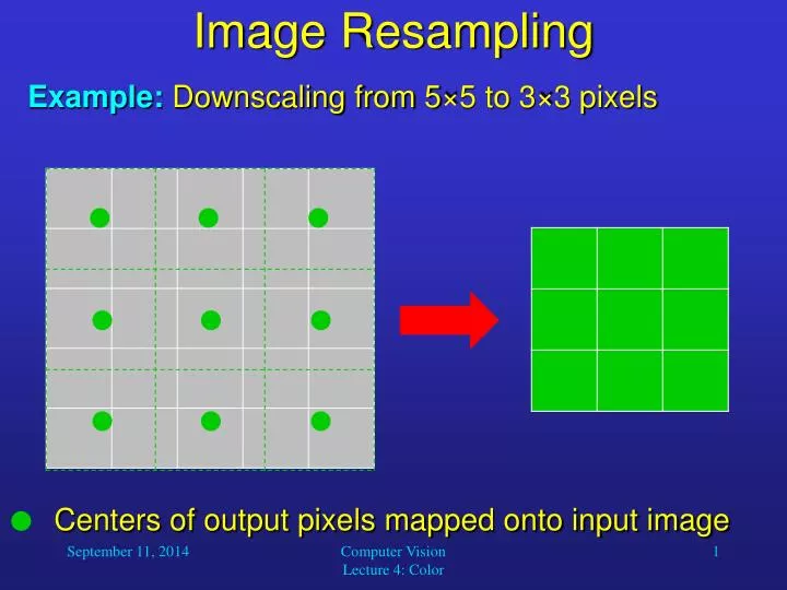
Image Resampling • Example: Downscaling from 5×5 to 3×3 pixels • Centers of output pixels mapped onto input image Computer Vision Lecture 4: Color
Image Resampling • Nearest-neighbor method: For each output pixel, intensity is taken from the input pixel whose center is closest to the mapped output pixel’s center. • Centers of output pixels mapped onto input image Computer Vision Lecture 4: Color
Image Resampling • Bilinear interpolation method: Consider the four closest neighbors (2×2) of each mapped output pixel. Then use linear interpolation in horizontal and vertical direction to determine output pixel intensity. • Bicubicinterpolation method: Consider the 16 closest neighbors (4×4) of each mapped output pixel. Then use cubic interpolation (polynomials of degree 3) in horizontal and vertical direction to determine output pixel intensity. • Many current image processing applications use bicubic interpolation. Computer Vision Lecture 4: Color
300 120 80 40 • Nearest neighbor • Bilinear interpolation • Bicubic interpolation Computer Vision Lecture 4: Color
Color Computer Vision Lecture 4: Color
Color • Our retina has three different types of color receptors. Their maximum responses occur for the colors red, green, and blue, respectively. Our color perception is entirely based on these three responses. Any two input spectra that create the same pattern of responses are perceived as identical colors. Computer Vision Lecture 4: Color
Color • How can we quantitatively describe a color? • As computer programmers, we usually treat colors as RGB triples. • The three components define the amount of red, green, and blue, respectively, whose combination results in the desired color on a computer screen. • Typically, each channel uses discrete values from 0 to 255. • The color space formed by all possible RGB values is also called the RGB cube. Computer Vision Lecture 4: Color
Color • The RGB color space is easy to use and represents color in the same way as the monitor requires it for its display. • However, for computer vision applications such as the recognition of objects, other color spaces are more useful. • We will discuss the HSI color model, standing for hue, saturation, and intensity. • These dimensions characterize important object properties more naturally as compared to the RGB components. Computer Vision Lecture 4: Color
Color • Hue is determined by the dominant wavelength in the spectral distribution of light wavelengths. • Saturation is the magnitude of the hue relative to other wavelengths. • It is defined as the amount of light at the dominant wavelength divided by the amount of light at all wavelengths. • Intensity is a measure of the overall amount of light within the visible spectrum. • It is a scale factor that is applied across the entire spectrum. Computer Vision Lecture 4: Color
Color • Hue • Saturation • Brightness Computer Vision Lecture 4: Color
Color • Hue is (ideally) independent of the lighting conditions and the distance between object and observer. It is thus a reliable parameter for object recognition. • Saturation decreases with the amount of particles between object and observer. We can use it to estimate our distance from a known object. • Intensity is the only variable that changes when the lighting conditions vary. It can be used to infer shading and, in turn, three-dimensional structure. Computer Vision Lecture 4: Color
Color • RGB HSI Computer Vision Lecture 4: Color
Conversion from RGB to HSI • It is not too difficult to convert RGB values into HSI values to facilitate color processing in computer vision applications. • First of all, we normalize the range of the R, G, and B components to the interval from 0 to 1. • For example, for 24-bit color information, this can be done by dividing each value by 255. • Then we compute the intensity I as • I = 1/3*(R + G + B). • Obviously, intensity also ranges from 0 to 1. Computer Vision Lecture 4: Color
Conversion from RGB to HSI • Then we compute the values r, g, b that are independent of intensity: • r = R/(R + G + B) • g = G/(R + G + B) • b = B/(R + G + B) • When we consider the RGB cube, then all possible triples (r, g, b) lie on a triangle with corners (1, 0, 0), (0, 1, 0), and (0, 0, 1). • We could call this the rgb-subspace of our RGB cube. Computer Vision Lecture 4: Color
green p - w p = (r, g, b) pr - w H red (pr) w = (1/3, 1/3, 1/3) (white) blue Conversion from RGB to HSI • The hue is the angle H from vector pr – w to vector p – w. • The saturation is the distance from w to p relative to the distance from w to the fully saturated color of the same hue as p (on the edge of the triangle). Computer Vision Lecture 4: Color
Conversion from RGB to HSI • Then we have: Since w = (1/3, 1/3, 1/3): And since pr = (1, 0, 0): Computer Vision Lecture 4: Color
Conversion from RGB to HSI • We can also compute: With the above formulas, including those for deriving r, g, and b from R, G, and B, we can determine an equation for computing H directly from R, G, and B: Computer Vision Lecture 4: Color
Conversion from RGB to HSI Note that when we use the arccos function to compute H, arccos always gives you a value between 0 and 180 degrees. However, H can assume values between 0 and 360 degrees. If B > G, then H must be greater than 180 degrees. Therefore, if B > G, just compute H as before and then take (360 degrees – H) as the actual hue value. Computer Vision Lecture 4: Color
Conversion from RGB to HSI The saturation is the distance on the triangle in the rgb-subspace from white relative to the distance from white to the fully saturated color with the same hue. Fully saturated colors are on the edges of the triangle. The derivation of the formula for saturation S is very lengthy, so we will just take a look at the result: Computer Vision Lecture 4: Color
Computer Vision Lecture 4: Color
Limitations of RGB and HSI Using three individual wavelengths to represent color can never cover the entire visible range of colors: Computer Vision Lecture 4: Color
Limitations of any Color Representation It is important to note (again) that our perception of an object’s color does not only depend on the frequency spectrum emitted from the object’s location. It also depends on the spectra of other objects or regions in the visual field. This mechanism called color constancy allows us to assign a color to a given object that is invariant to shading or illumination of the scene by varying light sources. Computer Vision Lecture 4: Color
Color Constancy Computer Vision Lecture 4: Color