Download
1 / 58
590 likes | 724 Views
Ben Gurion University of the Negev. www.bgu.ac.il/atomchip , www.bgu.ac.il/nanocenter. Physics 2 for Electrical Engineering. Lecturers: Daniel Rohrlich , Ron Folman Teaching Assistants: Ben Yellin, Yoav Etzioni Grader: Gady Afek.

E N D
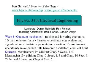
Ben Gurion University of the Negev www.bgu.ac.il/atomchip,www.bgu.ac.il/nanocenter Physics 2 for Electrical Engineering Lecturers: Daniel Rohrlich , Ron Folman Teaching Assistants: Ben Yellin, Yoav Etzioni Grader: Gady Afek Week 10. Maxwell’s equations – Introduction•The problem with Ampère’s law • Maxwell’s fix• • Stokes’s theorem Source: Halliday, Resnick and Krane, 5th Edition, Chap. 38.
(Gauss’s law) (Faraday’s law) (Ampère’s law) Introduction The set of four fundamental equations for E and B, together with the Lorentz force law FEM = q (E + v × B), sum up everything we have learned so far about electromagnetism!
Introduction This lecture and the next describe one of the great advances in the history of science, namely, how J. C. Maxwell discovered a problem with Ampère’s law, how he solved the problem, and how he was led to the amazing prediction of electromagnetic waves. These two lectures are is also more mathematical than the other lectures. We need the mathematics in order to analyze Maxwell’s work efficiently. We need two operators – the “curl” and the “divergence” – and corresponding theorems: “Stokes’s theorem” and the “divergence theorem”.
z S ∂S y Rutgers x Introduction New notation: If S denotes a surface (which may be curved), then ∂S denotes the boundary of the surface S:
I B ds I = 0 The problem with Ampère’s law We have seen that Ampère, building on Oersted’s discovery and on the law of Biot and Savart, postulated the law named after him:
(Ampère’s law) (Faraday’s law) The problem with Ampère’s law Now let’s compare Ampère’s law with Faraday’s law: With the new notation, we can write the left side of Faraday’s law as an integral over the closed loop ∂S, and the right side as an integral over any surface S bounded by the closed loop ∂S.
(Ampère’s law) (Faraday’s law) The problem with Ampère’s law Now let’s compare Ampère’s law with Faraday’s law: With the new notation, we can write the left side of Faraday’s law as an integral over the closed loop ∂S, and the right side as an integral over any surface S bounded by the closed loop ∂S. How do we know that the surface S on the right side can be any surface?
(Ampère’s law) (Faraday’s law) The problem with Ampère’s law Now let’s compare Ampère’s law with Faraday’s law: With the new notation, we can write the left side of Faraday’s law as an integral over the closed loop ∂S, and the right side as an integral over any surface S bounded by the closed loop ∂S. Can we write Ampère’s law this way?
The problem with Ampère’s law Yes, we can! With the new notation, we can write the left side of Ampère’s law as an integral over the closed loop ∂S, and the right side as an integral over any surface S bounded by the closed loop ∂S. Here J is the current density. (Ampère’s law)
The problem with Ampère’s law This is indeed what Ampère intended with his law, namely that the right side is the current flowing through any surface S bounded by the closed loop ∂Son the left side. However, there is a problem with Ampère’s law when we consider an electrical circuit with a capacitor in it.
–q ∂S q Surface S2 I Surface S1 The problem with Ampère’s law How do we apply Ampère’s law, to this electrical circuit?
–q ∂S B q r Surface S2 I Surface S1 The problem with Ampère’s law How do we apply Ampère’s law, to this electrical circuit? Let’s suppose the capacitor in this figure is charging (I = dq/dt > 0) and apply Ampère’s law to Surface S1: (2πr)B = μ0I, so B = μ0I/2πr .
–q ∂S q Surface S2 I Surface S1 The problem with Ampère’s law How do we apply Ampère’s law, to this electrical circuit? Let’s suppose the capacitor in this figure is charging (I = dq/dt > 0) and apply Ampère’s law to Surface S2: (2πr)B = 0, so B = 0 .
–q ∂S B q r Surface S2 I Surface S1 The problem with Ampère’s law How do we apply Ampère’s law, to this electrical circuit? Current flows through Surface S1. No current flows through Surface S2. Hence we have a μ0I/2πr = B = 0: CONTRADICTION!
–q ∂S B q r Surface S2 I Surface S1 The problem with Ampère’s law How do we apply Ampère’s law, to this electrical circuit? CAN WE FIX THIS CONTRADICTION?
–q q I ∂S The problem with Ampère’s law You may say, “This is silly. Ampère’s law is not like Faraday’s law, no matter what Ampère thought. Forget about S1 and S2! Just consider how much current flows through the closed loop ∂S.” Yes, but suppose the closed loop straddles the capacitor: How much current is flowing through the loop ∂S now?
Maxwell’s fix J. C. Maxwell noticed this problem with Ampère’s law. And there is another problem: In all of physics, interactions are mutual. Newton’s third law states that to every action there is an equal and opposite reaction. In electrostatics, a charge creates an electric field and an electric field accelerates a charge. In magnetostatics, a moving charge creates a magnetic field and a magnetic field accelerates a moving charge.
Maxwell’s fix J. C. Maxwell noticed this problem with Ampère’s law. And there is another problem: In all of physics, interactions are mutual. Newton’s third law states that to every action there is an equal and opposite reaction. In electrostatics, a charge creates an electric field and an electric field accelerates a charge. In magnetostatics, a moving charge creates a magnetic field and a magnetic field accelerates a moving charge. But according to Faraday’s law, a changing magnetic field creates an electric field…. Is this interaction mutual?
Maxwell’s fix J. C. Maxwell noticed this problem with Ampère’s law. And there is another problem: In all of physics, interactions are mutual. Newton’s third law states that to every action there is an equal and opposite reaction. In electrostatics, a charge creates an electric field and an electric field accelerates a charge. In magnetostatics, a moving charge creates a magnetic field and a magnetic field accelerates a moving charge. Maxwell speculated that a changing electric field could create a magnetic field.
–q ∂S B q r Surface S2 I Surface S1 Maxwell’s fix Maxwell’s speculation could save Ampère’s law! The capacitor in this figure is charging. If we consider Surface S1, there is a magnetic field B because of the current I through S1. If we consider Surface S2, there is a magnetic field B because of the changing electric field in the capacitor!
(Gauss’s law) (Faraday’s law) (Ampère’s law as modified by Maxwell) Maxwell’s fix This set of four fundamental equations for E and B, is called Maxwell’s equations!
–q ∂S B q r Surface S2 I Surface S1 Maxwell’s fix Let’s check that Maxwell’s modification of Ampère’s law, fixes the problem, for the case of a parallel- plate capacitor. If we consider Surface S1, we have (2πr)B = μ0I .
–q ∂S B q r Surface S2 I Surface S1 Maxwell’s fix Let’s check that Maxwell’s modification of Ampère’s law, fixes the problem, for the case of a parallel- plate capacitor. If we consider Surface S2, we have (2πr)B = μ0ε0 dΦE/dt. For a parallel-plate capacitor, it still equals μ0I!
Maxwell’s fix Let’s check that Maxwell’s modification of Ampère’s law, fixes the problem, for the case of a parallel-plate capacitor. If we consider Surface S1, we have (2πr)B = μ0I . If we consider Surface S2, we have (2πr)B = μ0ε0 dΦE/dt. For a parallel-plate capacitor of area A and plate separation d, ΦE = AE = AV/d = Aq/Cd, and C = ε0 A/d, so ΦE = qA/Cd = q/ε0. We get dΦE/dt = I/ε0 so (2πr)B = μ0ε0 dΦE/dt = μ0I! Note I = ε0 dΦE/dt is often called the displacement current.
Maxwell’s fix Without going into the details, we can already anticipate electromagnetic radiation: A changing electric flux will generate a transient magnetic field around it, which will generate a transient electric field, etc. etc. while the wave spreads through space.
E We will now develop the mathematical tools we need for analyzing Maxwell’s equations. We begin with the curl and Stokes’s theorem.
E The curl of a vector field E(x,y,z), written , is the following vector field: We can write it as a determinant:
E Example 1: Show that if for some function V(r).
E Example 1: Show that if for some function V(r). Answer: We assume , which means that Substituting these values into , we obtain We write : the curl of a gradient vanishes.
E Example 2: If r = (x,y,z), what is
E Example 2: If r = (x,y,z), what is Answer: i.e. r is a gradient, so
E Example 3: If B(r) = –yi+xj, what is
z B y x E Example 3: If B(r) = –yi+xj, what is Answer:
Stokes’s theorem Examples of tessellated surfaces:
Stokes’s theorem Examples of tessellated surfaces:
Stokes’s theorem There is even computer-aided basket weaving:
Stokes’s theorem Stokes’s theorem tells us how to compute an integral of the form around a closed loop∂S as an integral over a surface S which has ∂S as its boundary. For the proof of Stokes’s theorem, we assume that any surface S can be approximated arbitrarily well by triangulation, i.e. by reducing S to arbitrarily small triangles.
Stokes’s theorem Stokes’s theorem tells us how to compute an integral of the form around a closed loop∂S as an integral over a surface S which has ∂S as its boundary. Here is an example of a triangulated surface: S ∂S
Stokes’s theorem Stokes’s theorem tells us that around the closed loop∂S is equal to the sum over all the triangles in the surface S that has ∂S as its boundary. n-th triangle S ∂S
Stokes’s theorem To see why Stokes’s theorem is true, all we have to do is look at two neighboring triangles and at for each one:
Stokes’s theorem To see why Stokes’s theorem is true, all we have to do is look at two neighboring triangles and at for each one: The integrals on their common side sum to zero, because the directions of integration are opposite!
S ∂S Stokes’s theorem When we put all the triangles together, the only integrals that contribute (that are not paired with opposing integrals) are the integrals along ∂S !
Stokes’s theorem When we put all the triangles together, the only integrals that contribute (that are not paired with opposing integrals) are the integrals along ∂S ! Stokes’s theorem thus tells us that i.e. that theintegral along ∂S equals the sum of the contribution of each triangle. We will now compute the contribution of an infinitesimal triangle. In the limit of infinitely many triangles, the sum over triangles will become an integral over the surface S.
Stokes’s theorem 1. We will assume that each triangle is a right-angled triangle, since any triangle can be cut into two right-angled triangles. 2. We will place one corner of the triangle at a point (u,v) on a uv-plane, and assume E depends linearly on Δu and Δv (since the triangle is infinitesimally small). 3. We will use a lemma: If f(s) depends linearly on s, then the integral of f(s) on the interval from s1 to s2 equals i.e. the average of f(s1) and f(s2) times the separation s2 – s1.
f(s2) f(s) f(s1) s s1 s2 Stokes’s theorem 1. We will assume that each triangle is a right-angled triangle, since any triangle can be cut into two right-angled triangles. 2. We will place one corner of the triangle at a point (u,v) on a uv-plane, and assume E depends linearly on Δu and Δv (since the triangle is infinitesimally small). 3. The shaded area is
Ev(u,v+Δv) Ev(u,v) Eu(u,v) Eu(u+Δu,v) Stokes’s theorem So here is our right-angled triangle:
Stokes’s theorem If we apply our lemma to compute for this triangle, we obtain
Stokes’s theorem If we apply our lemma to compute for this triangle, we obtain
Stokes’s theorem If we apply our lemma to compute for this triangle, we obtain
Stokes’s theorem If we apply our lemma to compute for this triangle, we obtain