Download
1 / 54
540 likes | 550 Views
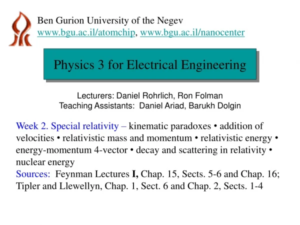
Ben Gurion University of the Negev. www.bgu.ac.il/atomchip , www.bgu.ac.il/nanocenter. Physics 3 for Electrical Engineering. Lecturers: Ron Folman, Daniel Rohrlich Teaching Assistants: Ben Yellin, Shai Bartal.

E N D
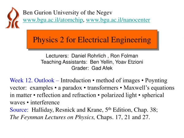
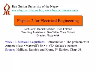
Ben Gurion University of the Negev www.bgu.ac.il/atomchip,www.bgu.ac.il/nanocenter Physics 3 for Electrical Engineering Lecturers: Ron Folman, Daniel Rohrlich Teaching Assistants: Ben Yellin, Shai Bartal Week 12. Quantum mechanics – propagation on a crystal lattice • Fermi level/momentum/energy • Kronig-Penney model and band gaps • GHZ and Bell’s theorem • quantum computing and cryptography. Sources: Feynman Lectures III, Chap. 13; Ashcroft and Mermin, Solid State Physics, Chap. 8; Tipler and Llewellyn, Sect. 10.6; selected papers to be distributed.
Propagation on a crystal lattice Some solids – including crystals and most metals – are periodic lattices. A periodic lattice obeys the Bragg condition for diffraction of waves from solids: d θ θ 2d sin θ = nλ
Propagation on a crystal lattice Some solids – including crystals and most metals – are periodic lattices. A periodic lattice obeys the Bragg condition for diffraction of waves from solids: d θ θ θ } d sin θ 2d sin θ = nλ
Electron diffraction Electrons on gold X-rays on zirconium oxide electrons
Neutron diffraction Diffraction of neutrons on a single NaCl crystal Diffraction of X-rays on a single NaCl crystal
V(x) Ion core d x Propagation on a crystal lattice To understand some generic features of electron conduction on a crystal lattice, let’s model a 1D crystal, i.e. a lattice with a periodic potential. The exact shape of the periodic potential will not matter.
Propagation on a crystal lattice To understand some generic features of electron conduction on a crystal lattice, let’s model a 1D crystal, i.e. a lattice with a periodic potential. The exact shape of the periodic potential will not matter. V(x) V(x) x d
Propagation on a crystal lattice We know how to solve Schrödinger’s equation for each barrier, but how do we connect up the solutions for all the barriers? V(x) V(x) x d
Propagation on a crystal lattice We know how to solve Schrödinger’s equation for each barrier, but how do we connect up the solutions for all the barriers? V(x) V(x) x d
Propagation on a crystal lattice Bloch’s theorem (1D): The eigenstates of where V(x) is periodic with period d, can be written where unk(x) is periodic with period d, i.e. unk(x+d) = unk(x). That is , every eigenstate has the property
Proof of Bloch’s theorem in three steps: 1. The operator shifts any function f(x) by d. Proof: 2. Therefore 3. Therefore the eigenstates of can be written as eigenstates of , which are
Fermi level/momentum/energy We will use Bloch’s theorem to find the relation between the momentum k and the energy E of an electron in a crystal lattice. But we ask first, How many momentum states are there in a crystal of length D? Assume that electron wave functions vanish outside the crystal. To be orthogonal, the eigenfunctions of must be in 1D, using “periodic boundary conditions” (x + D ↔ x). If electrons were bosons, we could put them all in the lowest-momentum state.
Fermi level/momentum/energy We will use Bloch’s theorem to find the relation between the momentum k and the energy E of an electron in a crystal lattice. But we ask first, How many momentum states are there in a crystal of length D? Assume that electron wave functions vanish outside the crystal. To be orthogonal, the eigenfunctions of must be in 1D, using “periodic boundary conditions” (x + D ↔ x). But electrons are fermions, so we can put just one in each momentum state.
Fermi level/momentum/energy In the ground state, all the momentum states are filled up to the state with the highest momentum magnitude kF, which is called the Fermi momentum. The corresponding highest energy EF, which equals in the simplest cases, is called the Fermi energy.
Fermi level/momentum/energy In 3D, the momentum states are vectors with components kx, ky, kz taking values We can think of triplets (kx,ky,kz), e.g. (4π/D,–16π/D,6π/D ), as points on a “reciprocal lattice”. When states are occupied up to the Fermi momentum, the triplets lie inside a ball of radius kF. The surface of this ball is called the Fermisurface. kz kF [From here.] kx ky
Compare Maxwell-Boltzmann and Fermi-Dirac statistics to see the effect of the Pauli exclusion principle: TF = 500 K
Compare Maxwell-Boltzmann and Fermi-Dirac statistics to see the effect of the Pauli exclusion principle: Average occupancy vs. average kinetic energy
Exercise: What is the minimum energy of a population of N fermions?
Exercise: What is the minimum energy of a population of N fermions? Solution: so and
Exercise: What is the minimum energy of a population of N fermions? Solution: so and The “density of states” dN/dEF is Exercise: Find the 2D versions of EF and dN/dEF. Exercise: Given that electron densities in metals are of order 1022/cm3, find the speed of the fastest electrons.
Kronig-Penney model and band gaps So far, we have not discussed E(p), the relation between the energy E and the momentum p = ħk of electrons in crystals. But E(p) has dramatic consequences. E E Allowed band E Forbidden band Allowed band k k Electron in crystal Free electron
Kronig-Penney model and band gaps So far, we have not discussed E(p), the relation between the energy E and the momentum p = ħk of electrons in crystals. But E(p) is remarkable, and has dramatic consequences. E E Allowed band Forbidden band EF Allowed band k k conductor Electron in crystal Free electron
Kronig-Penney model and band gaps So far, we have not discussed E(p), the relation between the energy E and the momentum p = ħk of electrons in crystals. But E(p) is remarkable, and has dramatic consequences. E E Allowed band EF Forbidden band Allowed band k k insulator Electron in crystal Free electron
Kronig-Penney model and band gaps So far, we have not discussed E(p), the relation between the energy E and the momentum p = ħk of electrons in crystals. But E(p) is remarkable, and has dramatic consequences. Where does the “band gap” come from? E E Allowed band EF Forbidden band Allowed band k k insulator Electron in crystal Free electron
V(x) -d d 2d 3d Kronig-Penney model and band gaps The “Kronig-Penney” model is a 1D lattice of square potential wells with lattice spacing is d. x
Kronig-Penney model and band gaps The “Kronig-Penney” model is a 1D lattice of square potential wells with lattice spacing is d. The energy E of an electron as a function of its wave number k is shown below for an electron in this lattice. Energy gaps appear when k = nπ/d. k 3π/d 2π/d 0 π/d
The gap arises from standing waves that resonate through the lattice at k = nπ/d. For n = 1, for example, the waves are The figure shows the spatial probability distribution of both waves. |ψ–|2 |ψ+|2 traveling wave x d
V(x) x d Prob. 8.1 in Solid State Physics by Ashcroft and Mermin is a mathematical analysis of band gaps in 1D. Assume a potential V(x) such that V(–x) = V(x) and V(±d/2) = 0 and V(x+d) = V(x). There are two scattering solutions, ψl(x) and ψr(x), with the following behaviors at x = ±d/2:
Prob. 8.1 in Solid State Physics by Ashcroft and Mermin is a mathematical analysis of band gaps in 1D. Assume a potential V(x) such that V(–x) = V(x) and V(±d/2) = 0 and V(x+d) = V(x). There are two scattering solutions, ψl(x) and ψr(x), with the following behaviors at x = ±d/2: and
We now define a general solution ψ(x) = Aψl(x) + Bψr(x) and impose two conditions: and Imposing these conditions on ψ(x) we can derive the following: and since in general rt* is pure imaginary and |r|2+|t|2 = 1, we can also derive where t = |t|eiδ . Now if |t| < 1, there are no solutions for k when Kd+δ ≈ nπ. This is the origin of the band gaps.
Exercise: For weak scattering (|t| ≈ 1, δ≈ 0), derive the width of the band gap. Solution: The gap occurs for cos Kd > |t|. Since |r|2+|t|2 = 1 and |t| ≈ 1, we can approximate |t| ≈ 1–|r|2 /2. The relevant values of K are those for which Kd ≈ nπ. For those values, we can approximate cos Kd as 1 – |Kd–nπ |2/2. Thus, the limits of the gap occur when |Kd±nπ| = |r|, i.e. when K = (|r|±nπ)/d. Since the energy is we have as the width of the band gap.
Electrons perform miracles! In superconductivity (which occurs at temperatures as high as 160 K), currents encounter no resistance. Electrical resistance suddenly vanishes as a superconductor is cooled below its critical temperature Tc. normal metal superconductor
Electrons perform miracles! In superconductivity (which occurs at temperatures as high as 160 K), currents encounter no resistance. Superconductors expel all magnetic flux (Meissner effect)
Electrons perform miracles! In superconductivity (which occurs at temperatures as high as 160 K), currents encounter no resistance. Superconductors expel all magnetic flux (Meissner effect) The explanation for superconductivity put forward by J. Bardeen, L. Cooper and J.R. Schrieffer [BCS] in the Physical Review106 (1957) 162 is based on “bosonic” pairs of electrons having k (with spin up) and –k (with spin down) that are far apart but interact via the lattice.
GHZ and Bell’s theorem Is the uncertainty principle a fundamental limit on what we can measure? Or can we evade it? Einstein and Bohr debated this question for years, and never agreed.
GHZ and Bell’s theorem Is the uncertainty principle a fundamental limit on what we can measure? Or can we evade it? Einstein and Bohr debated this question for years, and never agreed. Today we are certain that uncertainty will not go away. Quantum uncertainty is even the basis for new technologies such as quantum cryptology. It may be that the universe is not only stranger than we imagine, but also stranger than we can imagine.
GHZ and Bell’s theorem In 1935, after failing for years to defeat the uncertainty principle, Einstein argued that quantum mechanics is incomplete. The famous “EPR” paper
GHZ and Bell’s theorem In 1935, after failing for years to defeat the uncertainty principle, Einstein argued that quantum mechanics is incomplete. Note that [x, p] ≠ 0, but [x2–x1, p2+p1] = [x2, p2] – [x1, p1] = 0. That means we can measure the distance between two particles and their total momentum, to arbitrary precision. So we can measure either x2orp2 without affecting Particle 2 in any way, via a measurement on Particle 1 (and vice versa). That means both x2andp2 are simultaneously real. Quantum mechanics has no place for simultaneous x2 and p2 , so quantum mechanics is incomplete.
GHZ and Bell’s theorem Some reactions to the EPR argument: Bohr (1935) The uncertainty principle still applies. Pauli (1954) “One should no more rack one's brain about the problem of whether something one cannot know anything about exists all the same, than about the ancient question of how many angels are able to sit on the point of a needle. But it seems to me that Einstein's questions are ultimately always of this kind.” Bell (1964) Quantum mechanics contradicts EPR!
GHZ and Bell’s theorem We will consider a theorem similar to Bell’s, proved in 1988 by D. Greenberger, M. Horne, and A. Zeilinger (GHZ). It describes three spin-½ particles prepared in one laboratory and sent to three different laboratories, operated by Alice, Bob, and Claire. For simplicity, we assume the particles are not identical.
GHZ and Bell’s theorem Setting for Greenberger-Horne-Zeilinger (GHZ) paradox: Alice Claire Bob A B C time O space
GHZ and Bell’s theorem We will consider a theorem similar to Bell’s, proved in 1988 by D. Greenberger, M. Horne, and A. Zeilinger (GHZ). It describes three spin-½ particles prepared in one laboratory and sent to three different laboratories, operated by Alice, Bob, and Claire. For simplicity, we assume the particles are not identical. The spin state of the three particles is where and .
GHZ and Bell’s theorem Alice can measure on her system; Bob can measure on his system; Claire can measure on her system; where (Recall ) The result of each measurement can be 1 or –1. Note
GHZ and Bell’s theorem To prove: 1. 2. That is, Alice, Bob and Claire discover two rules: 1. 2.
GHZ and Bell’s theorem But now because CONTRADICTION!
GHZ and Bell’s theorem But now because CONTRADICTION! This contradiction arose because we tacitly assumed, with EPR, that observables have values whether we measure them or not.
Quantum computing and cryptography. Introducing…the qubit (quantum bit). Like an ordinary “classical” bit, a qubit has two states: But unlike an ordinary bit, a qubit can be in any superposition of these two states! Quantum “CNOT” gate:
Quantum computing and cryptography. Introducing…the qubit (quantum bit). Like an ordinary “classical” bit, a qubit has two states: But unlike an ordinary bit, a qubit can be in any superposition of these two states! In principle, a quantum computer, given a superposition of inputs, computes the final result for each input simultaneously. Therefore there is a great speed-up of the computation. (The problem is that the final results, as well, are superposed.) In 1994, P. Shor devised an algorithm for factoring large numbers into primes, using a quantum computer. It is exponentially faster than any classical computer.
Quantum computing and cryptography. Shor’s algorithm puts in jeopardy all codes based on the RSA encoding method, which is based on the difficulty of factoring large numbers into primes. But have no fear! תורת הקוונטים הקדימה תרופה למכה! There are quantum codes, and they are unbreakable!
“10001010100100010” +10010101011010100 100011111111110110 100011111111110110 –10010101011010100 “10001010100100010” Example of quantum cryptography: “the one-time pad”. Bob Alice