Download
1 / 28
350 likes | 599 Views
Kelvin Waves El Niño. October 22. C p. Sea surface. pycnocline. Barotropic Wave. Ocean’s response to changing winds external (or surface)waves. C p. Sea Surface. pycnocline. Baroclinic Wave. p increasing. Hi. Hi. p decreasing. divergence. Lo. pgf. Cf. C. Lo. convergence.

E N D
Kelvin WavesEl Niño October 22
Cp Sea surface pycnocline Barotropic Wave • Ocean’s response to changing winds • external (or surface)waves
Cp Sea Surface pycnocline Baroclinic Wave
p increasing Hi Hi p decreasing divergence Lo pgf Cf C Lo convergence pgf is balanced by Cf p increasing Hi v=0 Top View • Coastal Kelvin waves get trapped against horizontal boundary Side View
for baroclinic waves Wave Phase Speed: ~0.5 to 3 m/s for barotropc (external) waves • L: measure of how far a water parcel can travel before it is affected by Coriolis: • f is smallest near the equator and largest near the poles, L increases toward the equator, coastal waves are not trapped at the equator
pgf pgf pgf Divergence Convergence Lo Hi Lo Equator pgf pgf pgf C Equatorial Kelvin Waves • Equator acts like a coast, with water on either side Equatorial Kelvin Waves move only to the East Le ~250 km, C~3 m/s
Figure 14.10 in Stewart. Left: Horizontal currents associated with equatorially trapped waves generated by a bell-shaped displacement of the thermocline. Right: Displacement of the thermocline due to the waves. The figures show that after 20 days, the initial disturbance has separated into an westward propagating Rossby wave (left) and an eastward propagating Kelvin wave (right). From Philander et al. (1984).
Figure 14.4 in Stewart. Cross section of the Equatorial Undercurrent in the Pacific calculated from Modular Ocean Model with assimilated surface data (See §14.5). The section an average from 160°E to 170°E from January 1965 to December 1999. Stippled areas are westward flowing. From Nevin S. Fuckar.
τ(x) τ(x) z=0 surface 80 m pycnocline 300-400 m Eq. under current 180° El Niño “Normal” state – Trade Winds pile up water in west
El Niño τ(x) τ(x) z=0 surface 200 m 200 m pycnocline Eq. under current 180° El Nino state - Winds relax or even reverse in western and central Pacific – pycnocline flattens out, undercurrent stops
equator Change in Trade Winds generate Kelvin wave that propagates eastward, depressing the pycnocline as it goes
pyc. depressed pyc. uplifted upwelling shuts off In 2-3 months – Kelvin Wave hits the coast of South America, part of it reflects as a RossbyWave, part moves poleward as a coastal Kelvin wave
CKW California Current Rossby Wave Rossby Wave Humbolt Current Coastal Kelvin Waves (CKW) go all the way to Canada and Chile, altering Eastern Boundary Currents and shutting down upwelling – Also influence ACC
Figure 14.14 in Stewart. Tropical Atmosphere Ocean tao array of moored buoys operated by the NOAA Pacific Marine Environmental Laboratory with help from Japan, Korea, Taiwan, and France. Figure from NOAA Pacific Marine Environmental Laboratory.
TOPEX Animation • Animation of SSH form the TOPEX Altimeter http://topex-www.jpl.nasa.gov/gallery/videos.html
Southern Oscillation Figure 14.6 in Stewart. Correlation coefficient of annual-mean sea-level pressure with pressure at Darwin. The Southern Oscillation Index is sea-level pressure at Tahiti minus sea-level pressure at Darwin . From Trenberth and Shea (1987).
Figure 14.7 in Stewart. Normalized Southern Oscillation Index from 1951 to 1999. The normalized index is sea-level pressure anomaly at Tahiti divided by its standard deviation minus sea-level pressure anomaly at Darwin divided by its standard deviation. Then the difference is divided by the standard deviation of the difference. The means are calculated from 1951 to 1980. Monthly values of the index have been smoothed with a 5-month running mean. Strong El Niño events occurred in 1957–58, 1965–66, 1972–73, 1982–83, 1997–98. Data from NOAA.
Figure 14.8 in Stewart. Anomalies of sea-surface temperature (in °C) during a typical El Niño obtained by averaging data from El Niños between 1950 and 1973. Months are after the onset of the event. From Rasmusson and Carpenter (1982).
Figure 14.11 in Stewart. Sketch of regions receiving enhanced rain (dashed lines) or drought (solid lines) during an El Niño event. (0) indicates that rain changed during the year in which El Niño began, (+) indicates that rain changed during the year after El Niño began. From Ropelewski and Halpert (1987).
Figure 14.12 in Stewart. Changing patterns of convection in the equatorial Pacific during an El Niño, set up a pattern of pressure anomalies in the atmosphere (solid lines) which influence the extratropical atmosphere. From Rasmusson and Wallace (1983).
Figure 14.13 in Stewart. Correlation of yearly averaged rainfall averaged over all Texas each year plotted as a function of the Southern Oscillation Index averaged for the year. From Stewart (1994).