Download
1 / 30
300 likes | 398 Views
Least Squares Regression a view by Henry Mesa. Use the arrow keys on your keyboard to move the slides forward and backward. Here is another view that explains the reason for regression. We are interested in a particular variable, which we name Y for convenience, the response variable.

E N D
Least Squares Regression a view by Henry Mesa
Use the arrow keys on your keyboard to move the slides forward and backward.
Here is another view that explains the reason for regression. We are interested in a particular variable, which we name Y for convenience, the response variable. We are only considering the situation in which Y is normally distributed. The distribution of Y has some mean and standard deviation.
What we would like to do is introduce another variable, which we call the explanatory variable, X, in the hopes that by doing so I can minimize the standard deviation of Y, .
Here is a cute site, showing a ball drop that creates a normal distribution. http://www.ms.uky.edu/~mai/java/stat/GaltonMachine.html Ok, go to the next slide.
Let us look at three scenarios so you can understand what we are doing. Oh, my gosh, cute ball thing! Y Lets say that Y is the height of a male adult. The height of male adult is normally distributed, and a population standard deviation exists, yet the value is unknown to us. We will introduce another variable, called X, in the hope to reduce the variability of the original standard deviation. x1 X
What we are hoping for is that for each value of the variable X, we can only associate a small range of the Y variable, thus decreasing our variation. Y So, let us consider two different scenarios. Possible Range of values for Y associated with x1; 2 standard deviations long x1 X
A poor situation- There is a linear association but for each value of x, the possible values of Y associated with x is too large; in this case r will be a low value. Y Let us day that X, represents the age of an individual adult. That would not be a good predictor of adult height. Possible Range of values for Y associated with x1; 2 standard deviations long v x1 x5 x4 x2 x3 X
A great situation- There is a linear association but for each value of x, and the possible values of Y associated with each x value is very small; in this case r will have a high value. Y Let us say that X represents the length of an adult male foot. The height of an individual and their foot size should be highly correlated. v vc Thus, in this case, the variable X should allow for a better prediction of the variable Y. So for example, a foot print if found at a crime scene, we would expect a decent predictor of height for the person whose print we recovered. x1 x5 x4 x2 x3 X
You will notice that the variable Y, has a mean value, Y, but its value is not known to us. Y v x1 x5 x4 x2 x3 X
But we can use the y values from the ordered pairs to calculate y-hat, . Y v x1 x5 x4 x2 x3 X
To remind ourselves of what is occurring, here is a picture of the model. The variables X and Y are not perfectly associated, but there is a linear trend. The line consist of joining the infinitely many normal distributions, by going through each center. X x2 x1 Y
The hope is that the means of each distribution is different (the larger the difference the better) and that the overall standard deviation (the same for each distribution) is small, so as to emphasize the difference between the means. X x2 x1 Y
Furthermore, Y is a different value from all of the individual means, except for one of the means. X x2 x1 Y
Lastly the equation of the line is given by Where “beta-one” is the slope of the line, but in reality none of these values is known to us, so we must rely on the data to approximate the slope. Thus, the statistical formula is Where b1 is the slope of the line, and it is a statistic, and y-hat is the approximation for the individual means for each distribution. X v v x2 x1 The red line is the result of calculating the least squares regression line. While the green line is the “true” line. Y
So is our best estimate of Y and y-hat, . is our best estimate for the individual means for each distribution, yxi Y v x1 x5 x4 x2 x3 X
So basically, we know nothing about our population, and unlike chapter 6 section 1 of Moore McCabe, we also do not know . Y v x1 x5 x4 x2 x3 X
On that note, we introduce the “error” which is not an error in the everyday sense. Y v x1 x5 x4 x2 x3 X
Error = observed y – predicted y. Y Predicted data Observed data v x2 x1 x5 x4 x3 X
Now calculate all errors for each observed data values and sum the errors squared. Y Predicted data Observed data v x2 x1 x5 x4 x3 X
I think you would agree that we would like the least possible error (strongest association). Y Predicted data Observed data v x2 x1 x5 x4 x3 X
The “least squares” regression line. Notice that we are “squaring” each error and we have established we would like the sum of squared errors to be as small as possible in order to have a “strong” association. That is what the calculation for the equation is trying to do, minimize the squared errors! The least squares regression line.
Here is a fun fact. The mean of the observed y’s is Y The mean of is also , and I mean the same number! The average is the same for both sets. Predicted data Observed data v x2 x1 x5 x4 x3 X
So, r-squared is the ratio of our approximation of the variation of the observed y’s, versus the predicted y’s. Think of it this way. Variability is what we are trying to model; we want the variability of the predicted y’s (the model) to closely match the variability of the observed y’s
Y Measures variation in observed y’s. Do this for all observed y’s, square the difference, and add. v x2 x1 x5 x4 x3 X
Y Measures variation in predicted y’s. Do this for all predicted y’s, square the difference, and add. v x2 x1 x5 x4 x3 X
Y v Thus, the ratio, says what fraction of the total variation (approximation of the actual situation), can be matched using the least squares regression line and the variable X as the model. x2 x1 x5 x4 x3 X
Least Squares Regression a view by Henry Mesa