Download
1 / 30
340 likes | 514 Views
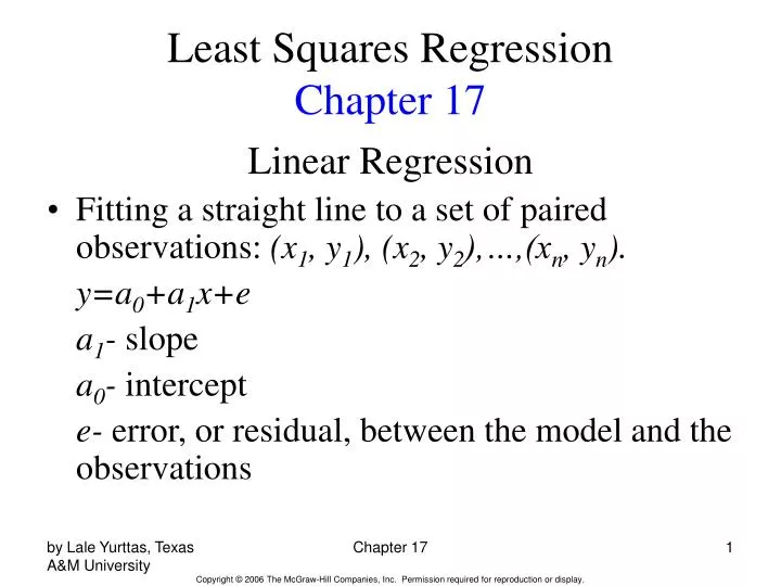
Least Squares Regression Chapter 17. Linear Regression Fitting a straight line to a set of paired observations: (x 1 , y 1 ), (x 2 , y 2 ),…,(x n , y n ). y=a 0 +a 1 x+e a 1 - slope a 0 - intercept e- error, or residual, between the model and the observations.

E N D
Least Squares RegressionChapter 17 Linear Regression • Fitting a straight line to a set of paired observations: (x1, y1), (x2, y2),…,(xn, yn). y=a0+a1x+e a1- slope a0- intercept e- error, or residual, between the model and the observations Chapter 17
Criteria for a “Best” Fit/ • Minimize the sum of the residual errors for all available data: n = total number of points • However, this is an inadequate criterion, so is the sum of the absolute values Chapter 17
Figure 17.2 Chapter 17
Best strategy is to minimize the sum of the squares of the residuals between the measured y and the y calculated with the linear model: • Yields a unique line for a given set of data. Chapter 17
List-Squares Fit of a Straight Line/ Normal equations, can be solved simultaneously Mean values
Figure 17.3 Chapter 17
Figure 17.4 Chapter 17
Figure 17.5 Chapter 17
“Goodness” of our fit/ If • Total sum of the squares around the mean for the dependent variable, y, is St • Sum of the squares of residuals around the regression line is Sr • St-Sr quantifies the improvement or error reduction due to describing data in terms of a straight line rather than as an average value. r2-coefficient of determination Sqrt(r2) – correlation coefficient
For a perfect fit Sr=0 and r=r2=1, signifying that the line explains 100 percent of the variability of the data. • For r=r2=0, Sr=St, the fit represents no improvement. Chapter 17
Polynomial Regression • Some engineering data is poorly represented by a straight line. For these cases a curve is better suited to fit the data. The least squares method can readily be extended to fit the data to higher order polynomials (Sec. 17.2). Chapter 17
General Linear Least Squares Minimized by taking its partial derivative w.r.t. each of the coefficients and setting the resulting equation equal to zero Chapter 17
InterpolationChapter 18 • Estimation of intermediate values between precise data points. The most common method is: • Although there is one and only one nth-order polynomial that fits n+1 points, there are a variety of mathematical formats in which this polynomial can be expressed: • The Newton polynomial • The Lagrange polynomial Chapter 17
Figure 18.1 Chapter 17
Newton’s Divided-Difference Interpolating Polynomials Linear Interpolation/ • Is the simplest form of interpolation, connecting two data points with a straight line. • f1(x) designates that this is a first-order interpolating polynomial. Slope and a finite divided difference approximation to 1st derivative Linear-interpolation formula Chapter 17
Figure 18.2 Chapter 17
Quadratic Interpolation/ • If three data points are available, the estimate is improved by introducing some curvature into the line connecting the points. • A simple procedure can be used to determine the values of the coefficients.
General Form of Newton’s Interpolating Polynomials/ Bracketed function evaluations are finite divided differences Chapter 18
Errors of Newton’s Interpolating Polynomials/ • Structure of interpolating polynomials is similar to the Taylor series expansion in the sense that finite divided differences are added sequentially to capture the higher order derivatives. • For an nth-order interpolating polynomial, an analogous relationship for the error is: • For non differentiable functions, if an additional point f(xn+1) is available, an alternative formula can be used that does not require prior knowledge of the function: x Is somewhere containing the unknown and he data Chapter 17
Lagrange Interpolating Polynomials • The Lagrange interpolating polynomial is simply a reformulation of the Newton’s polynomial that avoids the computation of divided differences: Chapter 17
As with Newton’s method, the Lagrange version has an estimated error of: Chapter 17
Figure 18.10 Chapter 17
Coefficients of an Interpolating Polynomial • Although both the Newton and Lagrange polynomials are well suited for determining intermediate values between points, they do not provide a polynomial in conventional form: • Since n+1 data points are required to determine n+1 coefficients, simultaneous linear systems of equations can be used to calculate “a”s. Chapter 17
Where “x”s are the knowns and “a”s are the unknowns. Chapter 17
Figure 18.13 Chapter 17
Spline Interpolation • There are cases where polynomials can lead to erroneous results because of round off error and overshoot. • Alternative approach is to apply lower-order polynomials to subsets of data points. Such connecting polynomials are called spline functions. Chapter 17
Figure 18.14 Chapter 17
Figure 18.15 Chapter 17
Figure 18.16 Chapter 17
Figure 18.17 Chapter 17