Download

1 / 107
1.08k likes | 1.35k Views
Finding Regulatory Signals in Genomic Sequences. Weeder ProFind. Giancarlo Mauri. Bioinformatics and Natural Computing Group Dipartimento di Informatica, Sistemistica e Comunicazione Università degli Studi di Milano-Bicocca. Gene Expression Data.

E N D
Finding Regulatory Signals inGenomic Sequences Weeder ProFind Giancarlo Mauri Bioinformatics and Natural Computing Group Dipartimento di Informatica, Sistemistica e Comunicazione Università degli Studi di Milano-Bicocca
Gene Expression Data • When and how much a gene is expressed under some given conditions (tissue, external stimuli, disease...) • We can group genes according to their expression profile • We can suspect a “common cause” for their expression
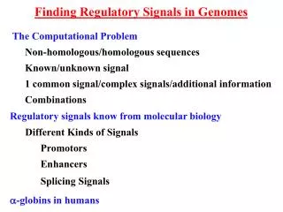
Transcription Factors • The expression of a gene starts with transcription from DNA to RNA • Transcription is modulated by dedicated proteins called transcription factors(TFs) • TFs bind to DNA in the regions surrounding the starting site of the gene (mostly upstream), and direct polymerases to the “right spot” to start transcription • Different effects: may enhance or block transcription
TF Transcription Starts TFBS
AND TF1 TF2 Transcription Starts TFBS
NOT TF1 TF2 Transcription Starts TFBS
TFs Binding Sites (TFBSs) Fundamental in regulatory analysis is the identification of potential TFBSs • Bound by transcription factors • Short degenerate sequences, 5-16 nucleotides long, (gaps possible but rare) • Each TF does not recognize a single fragment but a set of them (similar to each other) called signal or motif • Can be illustrated by profiles and/or consensi (computational models)
TFs Binding Sites (TFBSs) Fundamental in regulatory analysis is the identification of potential TFBSs • Bound by transcription factors • Short degenerate sequences, 5-16 nucleotides long, (gaps possible but rare) • Each TF does not recognize a single fragment but a set of them (similar to each other) called signal or motif • Can be illustrated by profiles and/or consensi (computational models)
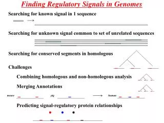
Finding TFBSs • We have a set of related genes: • similar expression profile • similar biological function • anything else.. • We take their upstream regulatory regions • If they are regulated by the same TF(s), then we should find its (their) binding sites in the sequences • We should find short patterns conserved in the sequences • We could use the detected TFBS to predict the behavior of a gene
Finding Novel TFBSs • Over-representation: • First, detect groups of similar oligos • Describe each group with a consensus or a profile (or in some other smart way) • Find the most over-represented groups If sequences were built at random and/or we picked sequences at random, the group should not appear with the same size/conservation
Finding Novel TFBSs • Most of early research has focused on the first point: how to detect the best groups (unfortunately, there are thousands of candidates) given simple score measures • Recent research has followed the second point: which is the best measure to tell “significant” groups from random similarities? • Is it expected or not, to find a group that is conserved? • Can we take advantage from the wealth of sequence data available?
Weeder : A tool for pattern discovery inGenomic Sequences Giancarlo Mauri* Giulio Pavesi* Graziano Pesole^ * Università degli Studi di Milano-Bicocca ^ Università degli Studi di Milano
References • G. Pavesi, G.Mauri, G.Pesole. An Algorithm for Finding Signals of Unknown Length in Unaligned DNA Sequences. Bioinformatics 17, S207-S214, 2001 • G.Pavesi, P.Mereghetti, G.Mauri, G.Pesole. WeederWeb: Discovery of Transcription Factor Binding Sites in a Set of Sequences from Co-Regulated Genes. Nucleic Acids Research Web Server Issue 2004, 32: W199-W203 • http://159.149.109.16:8080/weederWeb/
Weeder (2001) • Idea: instead of reducing the set of candidate patterns, reduce the set of possible matches for each pattern, trying to save a “significant” number of valid occurrences • Instead of searching exhaustively for patterns that occur in every sequence, we “short-sightedly” look for patterns that occur in a subset of them • The algorithm needs as input only a given error ratio e
Suffix Trees • A suffix tree is a data structure that exposes the internal structure of a string in a very deep and meaningful way • Suffix tree T for S = s1…sn • rooted directed tree • exactly n leaves numbered 1 to n • internal nodes with at least two sons • edges labeled by non empty substrings of S • labels out of the same node begin with different symbols • the concatenation of the edge labels on the path from the root to any leaf i exactly spells the suffix of S starting at position i, i.e., s1…sn
Suffix Trees • The same structure can be built also for a set of k sequences • To distinguish which sequence a suffix belongs to, it appends a different marker symbol, not occurring elsewhere, to each sequence in the set. • It is also possible to annotate each node of the tree with a k-bit string, where the i-th bit is set if the word spelled by the path ending at the node occurs in the i-th sequence.
G # C A C C $ A C A A G $ A A $ G # G $ A # G # # Suffix Trees Suffix tree for ACCA (end with $) and CCAAG (end with #)
Suffix Trees • A generalized suffix tree can be built in O(N) time and takes O(N) space, where N is the overall length of the sequences • Annotating it with the bit strings takes additional O(kN) time • Each pattern occurring in the strings is spelled by a path starting from the root of the tree • The time needed to search for a pattern depends only on the length of the pattern • The structure allows to implement recursively the exhaustive enumeration of all the candidate patterns of a given length • The time complexity is thus reduced to be exponential in the maximum number of mutations allowed (Sagot, 1998)
Searching for an Exact Pattern • Given a set of sequences and the annotated suffix tree, every pattern appearing in at least one sequence of the set is spelled by a unique path starting from the root • We match the symbols of pattern p along the unique path in the tree until • p is exhausted • In this case, the bit string on the next node on the path specifies which sequences p appears in • no more matches are possible
Searching for a Pattern with Mismatches • We can also search for a pattern p with at most e mismatches in a similar way. • We match p along different paths on the tree at the same time, keeping track of the number of mismatches encountered on each path. • Whenever the number of errors on a path is greater than e, we discard that path. • The sequences p appears in are given by the logical-OR of the bit strings corresponding to the different paths.
Searching for (M, e) Patterns • The algorithm starts with the empty pattern from the root of the tree, and recursively expands it • Let us suppose we have found on the tree the endpoints of paths corresponding to the occurrences of a pattern p=p1…pm in the sequences, where all the paths spell words within distance e from p, with m<M • If p occurs in at least q sequences, we try and expand it by one symbol
Searching for (M, e) Patterns • Expanding a pattern by one symbol • For each character b {A, C, G, T}, we match b against the next symbol on each path • If a path ends just before a node V of the tree, we match b against the first symbol on each edge leaving V • When we encounter a mismatch, we increase the previous error along the path by one • If the new error is greater than e, we discard the path
Searching for (M, e) Patterns • Once all paths have been checked, the surviving ones represent the approximate occurrences of p’=p1…pmb • If p’ occurs in at least q sequences, and is shorter than M, we expand p’ as well. Otherwise, we continue with p and the next character in
Searching for (M, e) Patterns • For example • It matches the first symbol on each edge leaving the root against A. • If A is valid, i.e., A occurs in at least q sequences, it is expanded to AA. • If also AA is valid, we move to AAA, and so on. • If it is not valid, we proceed to look for occurrences of AC. • In this method, patterns don’t have to occur exactly in the sequences.
Searching for (M, e) Patterns • The main drawback is that every pattern of length e satisfies the input constraints, since every other pattern of length e found in the tree is a valid occurrence for it • Thus, the method works well only for small values of e
e Searching for (M, e) Patterns At the beginning of the search, all paths of length e are valid
Searching for (M, e) Patterns • To apply the algorithm also to longer patterns with higher values of e, instead of reducing the set of patterns that have to be searched, we restrict the number of paths that have to be followed for each pattern. • That is, we narrow down the set of valid occurrences-the WEEDER algorithm.
Searching for Approximate Occurrences of Patterns • Problem Definition: • Given a set of k sequences on the alphabet= { A, C, G, T }, we want to find all(M, e) patterns • (M, e) patterns: patterns oflength Mthat occur withat most e mismatchesin at least qsequencesof the set
The Outline of WEEDER • WEEDER fixes an initial error ratio • Given a pattern p, a path is valid if the distance from p to the path is not greater than |p| • |p| is the length of the pattern • When we expand p by one symbol, the error threshold is set to (|p|+1)
0 4 8 12 16 = 0.25 1 2 3 4 Block Decomposition of a Pattern • Each block size is 1/ • Let p = p1…pm. We can see p as composed of m blocks
Valid Occurrences • For every pattern p = p1…pm, valid occurrences are words si+1…si+m occurring in the sequences for which: j {1,…, m} d(p1…pj, si+1…si+j) j • d(p1…pj, si+1…si+j) is the number of mismatches between p1…pj and si+1…si+j • si+1…si+m is a valid occurrence for p if it is a valid occurrence for all its prefixes {p1, p1p2, …, p1p2…pm-1}
q = 2, =0.25 S2: AGCTCA& S1: AATCACGC# S3: ATGCT% S4: ACTC$ An Example for WEEDER G & C A GCTCA& T C T % % ATCACGC# C # GC# # GC# T T C CA& GCT% $ TC$ A % $ C CACGC# A A& CGC# GCT% & $ CGC# &
ACTCA: error max =2. S1, S2, S4 contain ACTCA. ACTC ACTCA G & C A GCTCA& T T C % % ATCACGC# C GC# # GC# # CA& T T C TC$ GCT% $ A % C $ CACGC# A A& CGC# GCT% & $ CGC# & ACTC: error max =1. S1, S2, S4 contain ACTC. S2: AGCTCA& S1: AATCACGC# S3: ATGCT% S4: ACTC$
ACTCA ACTCAA G & C A GCTCA& T T C % % ATCACGC# C GC# # GC# # T T C CA& TC$ $ GCT% A % $ C CACGC# A A& CGC# GCT% & $ CGC# & ACTCAA: error max =2. S1, S2 contain ACTCAA. ACTCAC, ACTCAG, ACTCAT are also patterns. S1: AATCACGC# S2: AGCTCA& S4: ACTC$ S3: ATGCT%
Weeder (2001) • Given a pattern P = p1p2....pm, the algorithm can find all the valid occurrences of P (with at most |P| mutations), such that at most i mutations occur in the first i letters of the pattern • But: some occurrences of a pattern can be missed altogether • Are DNA signals always so polite to show up in “blocks-decomposed” form? • The answer is no, but we can use Weeder with a grain of salt
Using Weeder • Example: (15,4) pattern occurring in 20 sequences • Valid (block decomposed) possible occurrences: 829 • Total possible occurrences:1365 • Probability if “hitting” a possible occurrence in a sequence: phit=.61 • Probability of finding the pattern in every sequence: like trying to win the national lottery • If we search for patterns occurring in at least 10 sequences, the probability of “seeing” at least 10 times the pattern is: Phit(20,10) = .89
Using Weeder • Thus, we can use Weeder as a sieve, to filter the set of candidate patterns • All patterns that are found to occur in at least q of the sequences by Weeder can be searched again in the sequences, but this time with no restriction on the position of mismatches • We expect the number of patterns (random patterns other than the real signal) passed to the second phase to be much smaller than the original number (and no longer exponential)
Using Weeder • The probability of finding a pattern in a sequence depends on its length and the error ratio • The probability of finding a pattern in a set of sequences (and thus the choice of the quorum q for the first phase) depends on the number of sequences • The same approach can be applied also when the signal does not show up in each sequence
Using Weeder • When the signal to be found is expected to be short, the algorithm can be used in “exact” mode • For longer signal, the lower is the quorum q, the higher is the probability of finding the signal • But: also the number of patterns satisfying the input constraints is higher, and the program is slower • Users can choose a suitable trade-off between time and accuracy
Theoretical Time Complexity • Naïve approach: O(4men) • Suffix tree approach (Sagot, 1998): O(4emekn) • where n is the input size, m is the pattern length, and e is the number of mutations allowed • Weeder: O((1/)e4ekn) where e is the number of mutations occurring in the longest pattern found
Weeder Web • Weeder Web is a web interface to the Weeder algorithm, where all the parameters concerning the motifs are automatically set for the discovery of transcription factor binding sites • Although there is no pre-set limit on the length of the input sequences, feasible results can be obtained by submitting sequences of "typical" length for regulatory/promoter regions (i.e. from 500 to 5000 bps) • A priori, there's no limit on the number of sequences you can input. Also, for the moment we do not consider correlations among different motifs (i.e. cis-regulatory modules)
Weeder Web • All the statistical measures (background oligo frequencies, expected occurrences and so on) used to score/rank motifs and to post-process the output have been derived from the analysis of promoter/enhancer and 5'UTR regions only (taken from different organisms) • If you submit something else (i.e. 3'UTRs, coding regions, noncoding RNAs, and so on) the statistical evaluation probably will not be consistent with your data, and thus produce unreliable results • http://www.pesolelab.it/Tool/ind.php
Post-Processing • Real motifs have different degrees of variation in different positions • Some admit “any” nucleotide • Some are (almost) perfectly conserved • We should find “redundant” motifs among the highest-scoring ones • Pieces of a long motif should appear also in shorter results
Post-Processing • Look for “redundant” (either in length or in conservation) motifs in the reports of each run • Collect the instances of each one and build a frequency matrix • Scan the sequences looking for matches • Report the best matches (with no constraint on the substitutions allowed)
Assessment results Tompa et.al., Nat Biotechnol. 2005 Jan;23(1):137-44.
ProFind : A GA Approach to the Definitionof Regulatory Signals inGenomic Sequences Characterization of CAP and TATA-box through probability matrices with a genetic algorithm Giancarlo Mauri, Roberto Mosca and Giulio Pavesi Bioinformatics and Natural Computing Group Dipartimento di Informatica, Sistemistica e Comunicazione Università degli studi di Milano-Bicocca
TATA Box and CAP Binding Sites • A large number of genes present two characteristic signals: • TATA-box • 25-35 bp upstream of the TSS • When discovered it was given a TATA consensus • Bound by the TATA Binding Protein (TBP) part of a large complex of some 50 different proteins including TFIID and TFIIB • CAP (also called Initiator or Inr) • Straddles the TSS • Experimental evidence that it is bound by TFIID too • Previous characterization by Bucher [1990] with a CA[Py] consensus • Very strong positional preference for the two signals with respect to the TSS
Describing Binding Sites Frequency Matrix nij .........0........... ...CGTGCCATTTGTTGT... ...TCCTACAGTGCAGCA... ...TCACATATTATTGTC... ...GAAAGCAACAACTAA... ...TAAATCGTCAGTGTA... ...CCGACCAGAGTGAAA... ...GGGTTTGGTTTGATA... ...GCGTGCAGTTGTGAA... ...GTCGCCATATACACA... ...GTGGCCGTATGCGCT... .........0........... ...CGTGCCATTTGTTGT... ...TCCTACAGTGCAGCA... ...TCACATATTATTGTC... ...GAAAGCAACAACTAA... ...TAAATCGTCAGTGTA... ...CCGACCAGAGTGAAA... ...GGGTTTGGTTTGATA... ...GCGTGCAGTTGTGAA... ...GTCGCCATATACACA... ...GTGGCCGTATGCGCT...