Download
1 / 55
550 likes | 708 Views
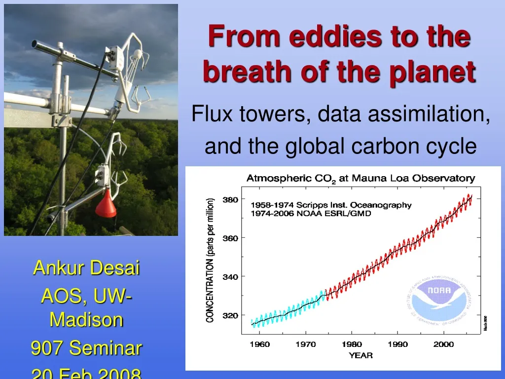
From eddies to the breath of the planet. Flux towers, data assimilation, and the global carbon cycle. Ankur Desai AOS, UW-Madison 907 Seminar 20 Feb 2008. PROLOGUE. What’s a meteorologist doing playing in the woods?. There’s gold in dem hills…. It’s alive…

E N D
From eddies to the breath of the planet Flux towers, data assimilation, and the global carbon cycle Ankur Desai AOS, UW-Madison 907 Seminar 20 Feb 2008
PROLOGUE What’s a meteorologist doing playing in the woods?
There’s gold in dem hills… • It’s alive… • Living organisms are strongly influenced by the atmosphere • And vice versa: living organisms play a large role in regulation of atmospheric composition, surface boundary conditions, air mass modification, and climate. • You can play too! • Land surface processes (AOS 532, Environmental Biophysics) • Boundary layers (AOS 773, Boundary layers, turbulence and micrometeorology) • Biogeochemistry (AOS 520, Bioclimatology) • Land-ocean-atmosphere interaction (AOS 425, Global Climate Processes; AOS 773, AOS 532)
Ask not what Earth system science can do for meteorologists… • Ask: What can meteorologists do for Earth system sciences? • Apply/develop novel tools for observing and modeling Earth systems • Atmosphere as the great mixer • We have the best toys • Physics based view of ecology • Ecology has traditionally been about local effects • Universal equations, parameters, paradigms are few • Rigorous mathematical analysis • Long history of working with large datasets and model output • Success with data assimilation
We really do have the best toys • Example: Atmospheric inversion • d Concentration / dt = Flux XTransport • If you know dC/dt and T, solve for F • A giant matrix inversion Source: NOAA ESRL Courtesy of A.S. Denning
Outline • What is the carbon cycle? • How do we observe it? • How can we use these observations to make better models? • What’s next?
ACT I Where we meet the carbon cycle and discover a breathing planet
Living planet, pt 1 • Sarmiento and Gruber, 2002, Physics Today
Living planet, pt 2 • Sarmiento and Gruber, 2002, Physics Today
Interannual variability • Peylin et al., 2005, GBC
An uncertain future • Friedlingstein et al., 2005, J. Clim
Moral • We need a way forward… • Can meteorology help ecology? • Can we go beyond local to global and universal? • Observations and models need a unifying framework • Use data assimilation, parameter estimation • Meteorologists know how to do this • Try to uncover controls, feedbacks, future sources, sinks and interactions • Counterintuitive results are likely
ACT II Much ado about eddies: Observing the exchange of a colorless, odorless gas
My friend eddy… • Tracers in boundary layer primarily transported by turbulence • Ensemble average turbulent equations of motion and tracer concentration provide information about the effect of random, chaotic turbulence on the evolution of mean tracer profiles with time • In a quasi-steady, homogenous surface layer, we can simplify this equation to infer the surface flux of a tracer
What we see • Lots of variation, some coherence WLEFtall tower Lost Creekwetland Sylvaniaold-growth Willow Creekhardwood
What we don’t see • Fluxes in low turbulence • Constant “footprint” • Components of flux • Energy balance
What we all see • Fluxnet database is growing!
What it means • Example: Carbon-water interactions in wetlands Source:B. Sulman
What it means • Micrometeorological forcing (air/soil temperature, light, water) explains much of hourly and daily fluxes • Synoptic forcing is important for understanding subweekly variability • Larger time lags exist in seasonal forcing (snow melt, growing degree days, canopy / micromet interaction…) • Fundamental rate reaction equations for photosynthesis, respiration, decomposition generally pan out • Long term variation is driven by vegetation type and age since disturbance - not easily observed by EC
What it doesn’t mean • Cannot directly observe / constrain flux components (e.g., GPP) • Parameters for many equations are not directly found from EC observations • Large heteroscedastic noise in EC observations and high frequency of low turbulence events makes long term continuous time series from EC hard to develop • Short term equations are non-linear, do not scale across averaging time • Long term ecosystem evolution equations are not well understood or known • Cannot simply scale or interpolate many flux measurements to get large region or global averages
Moral • Observations are a good thing • But they have no meaning without quality control • Moreover, they have no meaning without good interpretation • Can a model of land-atmosphere interaction help us out?
ACT III In which we decide how to build a better model* *Especially one that avoids Rube Goldberg syndrome
Why a model? • Complex, non-linear interactions are not easily understood with linear theory and empirical regression • Meteorological models are sensitive to initial conditions • Initial observation characterization/ensembles is key • But ecosystem models, like climate models, are more sensitive to boundary conditions (forcing) • Therefore, parameter estimation and trends in forcing become more important
Why data assimilation? • Old way: • Make a model • Guess some parameters • Compare to data • Publish the best comparisons • Attribute discrepancies to error • Be happy
Why data assimilation? • New way: • Constrain model(s) with observations • Find where model or parameters cannot explain observations • Learn something about fundamental interactions • Publish the discrepancies and knowledge gained • Work harder, be slightly less happy, but generate more knowledge
The basic idea of assimilation [A|B] = [AB] / [B] [P|D] = ( [D|P] [P] ) / [D] (parameters given data) = [ (data given parameters)× (parameters) ] / (data) Posterior = (Likelihood x Prior) / Normalizing Constraint
The basic idea of assimilation • Courtesy of D. Nychka, NCAR
Model of the day: Sipnet • A simplified model of ecosystem carbon / water and land-atmosphere interaction • Minimal number of parameters • Driven by meteorological forcing • Braswell et al., 2005, GCB • Sacks et al., 2006, GCB added snow
Hip-hop sensation: MC MC • Markov Chain Monte Carlo (MCMC) • A quasi-random walk in parameter space (Metropolis-Hastings algorithm) • From a prior parameter distribution, move in parameter space to minimize model-data RMS • ~100,000 iterations • Apply posterior parameters to get posterior “best” fit dataset and confidence • In Sipnet, NEE and LE fluxes from eddy covariance can be used to constrain the model using MCMC • Sipnet runs really fast (100 ms)
Case study 1: Sipnet Niwot Ridge • D. Moore, in review, Ag. For. Met.
Case study 1: Sipnet Niwot Ridge • D. Moore, in review, Ag. For. Met.
Case study 2: Sipnet WLEF • Part of ChEAS project… • 30m 122m 396m fluxes of CO2, H2O, H, u*
Caveat: Interannual variability • Ricciuto et al., in prep, Ag. For Met.
A brief word on other techniques • MCMC isn’t good for slow models and for real-time forecasting • Variational assimilation, Kalman filters, matrix inversion, etc… all have potential (mostly underutilized) • Ensemble Kalman Filter (EKF) is particularly appealing for constraining regional scale ecosystem models with atmospheric observations
Case study 3: ACME 2007 • Airborne Carbon in the Mountains Experiment
Case study 3: ACME 2007 CO2 MORNING UPWIND AFTERNOON DOWNWIND
Moral • Data assimilation and parameter estimation help us move beyond scratching heads over errors in observations and model logic • Formal ways to estimate fluxes and parameters are not necessarily hard to understand or implement • Assume large spread in prior parameters in land-atmosphere models • Long-term and high density datasets can have value beyond their original purposes
ACT IV Dénouement or Sequel: Where do we go from here?