Download

1 / 39
390 likes | 484 Views
CPE 400 / 600 Computer Communication Networks. Lecture 18. Chapter 4 Network Layer. slides are modified from J. Kurose & K. Ross. 4. 1 Introduction 4.2 Virtual circuit and datagram networks 4.3 What’s inside a router 4.4 IP: Internet Protocol Datagram format, IPv4 addressing, ICMP, IPv6

E N D
CPE 400 / 600Computer Communication Networks Lecture 18 Chapter 4Network Layer slides are modified from J. Kurose & K. Ross
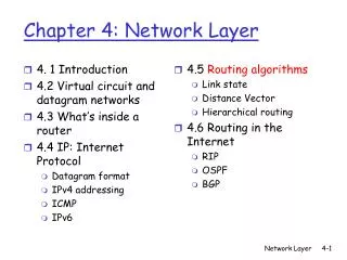
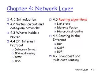
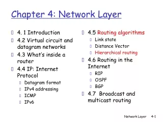
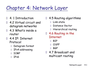
4. 1 Introduction 4.2 Virtual circuit and datagram networks 4.3 What’s inside a router 4.4 IP: Internet Protocol Datagram format, IPv4 addressing, ICMP, IPv6 4.5 Routing algorithms Link state, Distance Vector, Hierarchical routing 4.6 Routing in the Internet RIP, OSPF, BGP 4.7 Broadcast and multicast routing Chapter 4: Network Layer Network Layer
5 3 5 2 2 1 3 1 2 1 x z w y u v Graph abstraction Graph: G = (N,E) N = set of routers = { u, v, w, x, y, z } E = set of links ={ (u,v), (u,x), (v,x), (v,w), (x,w), (x,y), (w,y), (w,z), (y,z) } cost could always be 1, or inversely related to bandwidth, or inversely related to congestion c(x,x’) = cost of link (x,x’) Cost of path (x1, x2, x3,…, xp) = c(x1,x2) + c(x2,x3) + … + c(xp-1,xp) Network Layer
Dijkstra’s algorithm net topology, link costs known to all nodes accomplished via “link state broadcast” all nodes have same info computes least cost paths from one node (‘source”) to all other nodes gives forwarding table for that node iterative: after k iterations, know least cost path to k destinations Notation: c(x,y): link cost from node x to y; = ∞ if not direct neighbors D(v): current value of cost of path from source to dest. v p(v): predecessor node along path from source to v N': set of nodes whose least cost path definitively known A Link-State Routing Algorithm Network Layer
Dijsktra’s Algorithm 1 Initialization: 2 N' = {u} 3 for all nodes v 4 if v adjacent to u 5 then D(v) = c(u,v) 6 else D(v) = ∞ 7 8 Loop 9 find w not in N' such that D(w) is a minimum 10 add w to N' 11 update D(v) for all v adjacent to w and not in N' : 12 D(v) = min( D(v), D(w) + c(w,v) ) 13 /* new cost to v is either old cost to v or known 14 shortest path cost to w plus cost from w to v */ 15 until all nodes in N' Network Layer
5 3 5 2 2 1 3 1 2 1 x z w u y v Dijkstra’s algorithm: example D(v),p(v) 2,u 2,u 2,u D(x),p(x) 1,u D(w),p(w) 5,u 4,x 3,y 3,y D(y),p(y) ∞ 2,x Step 0 1 2 3 4 5 N' u ux uxy uxyv uxyvw uxyvwz D(z),p(z) ∞ ∞ 4,y 4,y 4,y Network Layer
x z w u y v destination link (u,v) v (u,x) x y (u,x) (u,x) w z (u,x) Dijkstra’s algorithm: example (2) Resulting shortest-path tree from u: Resulting forwarding table in u: Network Layer
4.5 Routing algorithms Link state Distance Vector Hierarchical routing 4.6 Routing in the Internet RIP OSPF BGP Lecture 18: Outline Network Layer
Distance Vector Algorithm Bellman-Ford Equation (dynamic programming) Define dx(y) := cost of least-cost path from x to y Then dx(y) = min {c(x,v) + dv(y) } where min is taken over all neighbors v of x v Network Layer
5 3 5 2 2 1 3 1 2 1 x z w u y v Bellman-Ford example Clearly, dv(z) = 5, dx(z) = 3, dw(z) = 3 B-F equation says: du(z) = min { c(u,v) + dv(z), c(u,x) + dx(z), c(u,w) + dw(z) } = min {2 + 5, 1 + 3, 5 + 3} = 4 Node that achieves minimum is next hop in shortest path ➜ forwarding table Network Layer
Distance Vector Algorithm • Dx(y) = estimate of least cost from x to y • Node x knows cost to each neighbor v: c(x,v) • Node x maintains distance vector Dx = [Dx(y): y є N ] • Node x also maintains its neighbors’ distance vectors • For each neighbor v, x maintains Dv = [Dv(y): y є N ] • From time-to-time, each node sends its own distance vector estimate to neighbors • When a node x receives new DV estimate from neighbor, it updates its own DV using B-F equation: • Under minor, natural conditions, the estimate Dx(y) converge to the actual least costdx(y) Dx(y) ← minv{c(x,v) + Dv(y)} for each node y ∊ N Network Layer
Iterative, asynchronous: each local iteration caused by: local link cost change DV update message from neighbor Distributed: each node notifies neighbors only when its DV changes neighbors then notify their neighbors if necessary wait for (change in local link cost or msg from neighbor) recompute estimates if DV to any dest has changed, notify neighbors Distance Vector Algorithm Each node: Network Layer
cost to x y z x 0 2 7 y from ∞ ∞ ∞ z ∞ ∞ ∞ 2 1 7 z x y Dx(z) = min{c(x,y) + Dy(z), c(x,z) + Dz(z)} = min{2+1 , 7+0} = 3 Dx(y) = min{c(x,y) + Dy(y), c(x,z) + Dz(y)} = min{2+0 , 7+1} = 2 node x table cost to x y z x 0 2 3 y from 2 0 1 z 7 1 0 node y table cost to x y z x ∞ ∞ ∞ 2 0 1 y from z ∞ ∞ ∞ node z table cost to x y z x ∞ ∞ ∞ y from ∞ ∞ ∞ z 7 1 0 time Network Layer
cost to x y z x 0 2 7 y from ∞ ∞ ∞ z ∞ ∞ ∞ 2 1 7 z x y Dx(z) = min{c(x,y) + Dy(z), c(x,z) + Dz(z)} = min{2+1 , 7+0} = 3 Dx(y) = min{c(x,y) + Dy(y), c(x,z) + Dz(y)} = min{2+0 , 7+1} = 2 node x table cost to cost to x y z x y z x 0 2 3 x 0 2 3 y from 2 0 1 y from 2 0 1 z 7 1 0 z 3 1 0 node y table cost to cost to cost to x y z x y z x y z x ∞ ∞ x 0 2 7 ∞ 2 0 1 x 0 2 3 y y from 2 0 1 y from from 2 0 1 z z ∞ ∞ ∞ 7 1 0 z 3 1 0 node z table cost to cost to cost to x y z x y z x y z x 0 2 7 x 0 2 3 x ∞ ∞ ∞ y y 2 0 1 from from y 2 0 1 from ∞ ∞ ∞ z z z 3 1 0 3 1 0 7 1 0 time Network Layer
1 4 1 50 x z y Distance Vector: link cost changes • Link cost changes: • node detects local link cost change • updates routing info, recalculates distance vector • if DV changes, notify neighbors At time t0, y detects the link-cost change, updates its DV, and informs its neighbors. At time t1, z receives the update from y and updates its table. It computes a new least cost to x and sends its neighbors its DV. At time t2, y receives z’s update and updates its distance table. y’s least costs do not change and hence y does not send any message to z. “good news travels fast” Network Layer
60 4 1 50 x z y Distance Vector: link cost changes • Link cost changes: • good news travels fast • bad news travels slow - “count to infinity” problem! • 44 iterations before algorithm stabilizes • Poisoned reverse: • If Z routes through Y to get to X : • Z tells Y its (Z’s) distance to X is infinite (so Y won’t route to X via Z) • will this completely solve count to infinity problem? Network Layer
Message complexity LS: with n nodes, E links, O(nE) msgs sent DV: exchange between neighbors only convergence time varies Speed of Convergence LS: O(n2) algorithm requires O(nE) msgs may have oscillations DV: convergence time varies may be routing loops count-to-infinity problem Robustness: what happens if router malfunctions? LS: node can advertise incorrect link cost each node computes only its own table DV: node can advertise incorrect path cost each node’s table used by others error propagate thru network Comparison of LS and DV algorithms Network Layer
4.5 Routing algorithms Link state Distance Vector Hierarchical routing 4.6 Routing in the Internet RIP OSPF BGP Lecture 18: Outline Network Layer
Hierarchical Routing • Our routing study thus far - idealization • all routers identical • network “flat” • … not true in practice • scale: with 200 million destinations: • can’t store all dest’s in routing tables! • routing table exchange would swamp links! • administrative autonomy • internet = network of networks • each network admin may want to control routing in its own network Network Layer
aggregate routers into regions, “autonomous systems” (AS) routers in same AS run same routing protocol “intra-AS” routing protocol routers in different AS can run different intra-AS routing protocol Gateway router Direct link to router in another AS Hierarchical Routing Network Layer
forwarding table configured by both intra- and inter-AS routing algorithm intra-AS sets entries for internal dests inter-AS & intra-As sets entries for external dests 3a 3b 2a AS3 AS2 1a 2c AS1 2b 3c 1b 1d 1c Inter-AS Routing algorithm Intra-AS Routing algorithm Forwarding table Interconnected ASes Network Layer
suppose router in AS1 receives datagram destined outside of AS1: router should forward packet to gateway router, but which one? AS1 must: learn which dests are reachable through AS2, which through AS3 propagate this reachability info to all routers in AS1 Job of inter-AS routing! 3a 3b 2a AS3 AS2 1a AS1 2c 2b 3c 1b 1d 1c Inter-AS tasks Network Layer
2c 2b 3c 1b 1d 1c Example: Setting forwarding table in router 1d • suppose AS1 learns (via inter-AS protocol) that subnet x reachable via AS3 (gateway 1c) but not via AS2. • inter-AS protocol propagates reachability info to all internal routers. • router 1d determines from intra-AS routing info that its interface I is on the least cost path to 1c. • installs forwarding table entry (x,I) … x 3a 3b 2a AS3 AS2 1a AS1 Network Layer
3a 3b 2a AS3 AS2 1a AS1 2c 2b 3c 1b 1d 1c Example: Choosing among multiple ASes • now suppose AS1 learns from inter-AS protocol that subnet x is reachable from AS3 and from AS2. • to configure forwarding table, router 1d must determine towards which gateway it should forward packets for dest x. • this is also job of inter-AS routing protocol! … … x Network Layer
Determine from forwarding table the interface I that leads to least-cost gateway. Enter (x,I) in forwarding table Use routing info from intra-AS protocol to determine costs of least-cost paths to each of the gateways Learn from inter-AS protocol that subnet x is reachable via multiple gateways Hot potato routing: Choose the gateway that has the smallest least cost Example: Choosing among multiple ASes • now suppose AS1 learns from inter-AS protocol that subnet x is reachable from AS3 and from AS2. • to configure forwarding table, router 1d must determine towards which gateway it should forward packets for dest x. • this is also job of inter-AS routing protocol! • hot potato routing: send packet towards closest of two routers. Network Layer
4.5 Routing algorithms Link state Distance Vector Hierarchical routing 4.6 Routing in the Internet RIP OSPF BGP Lecture 18: Outline Network Layer
Intra-AS Routing • also known as Interior Gateway Protocols (IGP) • most common Intra-AS routing protocols: • RIP: Routing Information Protocol • OSPF: Open Shortest Path First • IGRP: Interior Gateway Routing Protocol (Cisco proprietary) Network Layer
u v destinationhops u 1 v 2 w 2 x 3 y 3 z 2 w x z y C A D B RIP ( Routing Information Protocol) • distance vector algorithm • included in BSD-UNIX Distribution in 1982 • distance metric: # of hops (max = 15 hops) From router A to subnets: Network Layer
RIP advertisements • distance vectors: exchanged among neighbors every 30 sec via Response Message (also called advertisement) • each advertisement: list of up to 25 destination subnets within AS Network Layer
RIP: Example z w x y A D B C Destination Network Next Router Num. of hops to dest. w A 2 y B 2 z B 7 x -- 1 …. …. .... Routing/Forwarding table in D Network Layer
z w x y A D B C RIP: Example Dest Next hops w - 1 x - 1 z C 4 …. … ... Advertisement from A to D Destination Network Next Router Num. of hops to dest. w A 2 y B 2 z B A 7 5 x -- 1 …. …. .... Routing/Forwarding table in D Network Layer
RIP: Link Failure and Recovery If no advertisement heard after 180 sec --> neighbor/link declared dead • routes via neighbor invalidated • new advertisements sent to neighbors • neighbors in turn send out new advertisements (if tables changed) • link failure info quickly (?) propagates to entire net • poison reverse used to prevent ping-pong loops (infinite distance = 16 hops) Network Layer
routed routed RIP Table processing • RIP routing tables managed by application-level process called route-d (daemon) • advertisements sent in UDP packets, periodically repeated Transprt (UDP) Transprt (UDP) network forwarding (IP) table network (IP) forwarding table link link physical physical Network Layer
4.5 Routing algorithms Link state Distance Vector Hierarchical routing 4.6 Routing in the Internet RIP OSPF BGP Lecture 18: Outline Network Layer
OSPF (Open Shortest Path First) • “open”: publicly available • uses Link State algorithm • LS packet dissemination • topology map at each node • route computation using Dijkstra’s algorithm • OSPF advertisement carries one entry per neighbor router • advertisements disseminated to entire AS (via flooding) • carried in OSPF messages directly over IP (rather than TCP or UDP Network Layer
OSPF “advanced” features (not in RIP) • security: all OSPF messages authenticated (to prevent malicious intrusion) • multiple same-cost paths allowed (only one path in RIP) • For each link, multiple cost metrics for different TOS (e.g., satellite link cost set “low” for best effort; high for real time) • integrated uni- and multicast support: • Multicast OSPF (MOSPF) uses same topology data base as OSPF • hierarchical OSPF in large domains. Network Layer
Hierarchical OSPF Network Layer
Hierarchical OSPF • two-level hierarchy: local area, backbone. • Link-state advertisements only in area • each nodes has detailed area topology; only know direction (shortest path) to nets in other areas. • area border routers:“summarize” distances to nets in own area, advertise to other Area Border routers. • backbone routers: run OSPF routing limited to backbone. • boundary routers: connect to other AS’s. Network Layer
Routing algorithms Link state Distance Vector Hierarchical routing Routing in the Internet RIP OSPF Lecture 18: Summary Network Layer