Download

1 / 38
390 likes | 521 Views
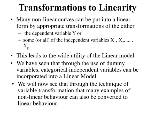
Unit 5: Transformations to achieve linearity. The S-030 roadmap: Where’s this unit in the big picture?. Unit 1: Introduction to simple linear regression. Unit 2: Correlation and causality. Unit 3: Inference for the regression model. Building a solid foundation. Unit 5:

E N D
The S-030 roadmap: Where’s this unit in the big picture? Unit 1: Introduction to simple linear regression Unit 2: Correlation and causality Unit 3: Inference for the regression model Building a solid foundation Unit 5: Transformations to achieve linearity Unit 4: Regression assumptions: Evaluating their tenability Mastering the subtleties Adding additional predictors Unit 6: The basics of multiple regression Unit 7: Statistical control in depth: Correlation and collinearity Generalizing to other types of predictors and effects Unit 9: Categorical predictors II: Polychotomies Unit 8: Categorical predictors I: Dichotomies Unit 10: Interaction and quadratic effects Pulling it all together Unit 11: Regression modeling in practice
In this unit, we’re going to learn about… • What happens if we fit a linear regression model to data that are nonlinearly related? • Alternative statistical models that are useful for nonlinear relationships • Logarithms—a brief refresher • The effects of logarithmic transformation • Other nonlinear relationships that can be modeled using logarithmic transformations • What’s the difference between taking logarithms to base 2, 10 and e? • Interpreting the regression of Y on log(X) • Interpreting the regression of log(Y) on X • Interpreting the regression of log(Y) on log(X) • How should we select among alternative transformation options: The Rule of the Bulge
The 10th Grade Math MCAS: % Scoring in the “Advanced” range Predictor Outcome The UNIVARIATE Procedure Variable: HOME Location Variability Mean 426.7553 Std Deviation 128.62042 Median 384.1250 Variance 16543 Mode 355.0000 Range 633.00000 The UNIVARIATE Procedure Variable: PCTADV Location Variability Mean 36.63636 Std Deviation 14.19603 Median 36.00000 Variance 201.52727 Mode 38.00000 Range 60.00000 Stem Leaf # Boxplot 8 8 1 * 8 7 5 1 0 7 14 2 0 6 558 3 0 6 0 1 | 5 699 3 | 5 244 3 | 4 5678 4 +-----+ 4 00012222234 11 | + | 3 55566666777778888899 20 *-----* 3 001222333334444 15 +-----+ 2 7 1 | 2 4 1 | ----+----+----+----+ Stem Leaf # Boxplot 7 1 1 | 6 59 2 | 6 12 2 | 5 5678 4 | 5 12344 5 | 4 57 2 | 4 1223344 7 +-----+ 3 6678888999 10 *--+--* 3 011223334 9 | | 2 567778899 9 +-----+ 2 011123344 9 | 1 56799 5 | 1 1 1 | ----+----+--- n = 66 ID DISTRICT HOME PCTADV L2HOME 1 AMESBURY 341.75 33 8.41680 2 ANDOVER 556.75 56 9.12089 3 ARLINGTON 476.00 44 8.89482 4 ASHLAND 390.00 38 8.60733 5 BELLINGHAM 308.00 15 8.26679 6 BELMONT 675.00 54 9.39874 7 BEVERLY 385.00 38 8.58871 8 BILLERICA 365.00 34 8.51175 9 BRAINTREE 375.00 39 8.55075 10 BROCKTON 269.90 11 8.07628 11 BURLINGTON 397.00 43 8.63300 12 CAMBRIDGE 749.00 23 9.54882 13 CANTON 472.50 41 8.88417 14 CHELMSFORD 360.45 38 8.49366 15 DANVERS 389.95 31 8.60715 16 DEDHAM 383.25 28 8.58214 17 DRACUT 296.25 27 8.21067 18 DUXBURY 537.50 55 9.07012 . . . Wellesley Cambridge Newton, Lexington Wellesley Brockton RQ: Is the percentage of 10th graders scoring in the advanced range on the math MCAS primarily a function of a district’s socioeconomic status?
Side Note: Percent Difference vs. Percentage Point Difference District Noname Percent Advanced: 10% Mandated to increase percent advanced by: 2 percentage points: Target rate for percent advanced? 10 percent: Target rate for percent advanced? 50 percent: Target rate for percent advanced? 5 percentage points: Target rate for percent advanced? 5 percentage points: Target rate for percent advanced? 7 percentage points: Target rate for percent advanced? 100 percent: Target rate for percent advanced? A percentage point difference is an arithmetic difference between two percentages. A percent difference is a proportional difference that is relative to a particular starting value.
What’s the relationship between PctAdv and Home Prices? Cambridge Cambridge The REG Procedure Dependent Variable: PCTADV Root MSE 9.11982 R-Square 0.5936 Dependent Mean 36.63636 Adj R-Sq 0.5873 Parameter Estimates Parameter Standard Variable DF Estimate Error t Value Pr > |t| Intercept 1 0.34532 3.91746 0.09 0.9300 HOME 1 0.08504 0.00879 9.67 <.0001 If the assumptions held (which they don’t!), we could interpret the slope coefficient as follows: Each $1000 difference in median home price is associated, on average, with a .085 percentage point difference in the percent of students scoring in the advanced category on MCAS. or $10,000 difference → .85 percentage point difference or $100,000 difference → 8.5 percentage point difference
What happens if we set aside Cambridge? Regression line with Cambridge The REG Procedure Dependent Variable: PCTADV Root MSE 7.37525 R-Square 0.7346 Dependent Mean 36.84615 Adj R-Sq 0.7304 Parameter Standard Variable DF Estimate Error t Value Pr > |t| Intercept 1 -4.86330 3.28861 -1.48 0.1442 HOME 1 0.09888 0.00743 13.20 <.0001
What happens when we fit a linear model to a non-linear relationship? More positive residuals (under-predicting) More positive residuals (under-predicting) More negative residuals (over-predicting) More negative residuals (over-predicting) More negative residuals (over-predicting) More negative residuals (over-predicting)
What alternative statistical model might be useful here? What kind of population model would have given rise to these sample data? The effect of HOME prices is larger when HOME prices are low and smaller when HOME prices are high
Logarithmic transformations in everyday life 1998 CPS Octave +110 (doubling) 1 M-Systems’ original 16 mb “disgo,” considered the first USB flash drive +220 (doubling) 2 Amplitude SW Richter +440 (doubling) 3 Greece, 1999 1,000,000 6.0 Japan, 1995 10,000,000 7.0 SF, 1906 100,000,000 8.0 Sumatra, 2004 1,000,000,000 9.0 Musical scales Flash drives, then and now Richter scale Each new generation doubles in storage capacity 16 32 64 128 256 512 1024 (1GB) 2G 4G 8G 16G … Up 1 octave = doubling of CPS Up 1 Richter = 10 fold ASW
Understanding Logarithms 1 2 4 8 16 32 64 Raw Log2 0 1 2 3 4 5 6 These are the logarithms For more on logarithms: Dallal, Logarithms, part I Each 1 unit increase in a base-2 logarithm represents a doubling of x Each 1 unit increase in a base-10 logarithm represents a 10-fold increase in x The power identifies the logarithmbase(x) because raising the base to that power yields x So…taking logs spreads out the distance between small values and compresses the distance between large values
Understanding the effects of logarithmic transformation in the MCAS data Wellesley ($875 9.77) One log unit Westwood ($600 9.23) One log unit Brockton ($269.9 8.07) Double of the raw: 512(2) = 1024 Double of the raw: 256(2) = 512 Gapminder
What happens if we regress PctAdv on log2(HOME)? ^ L2HOME PCTADV Home 256 8.0 13.48 362 8.5 30.28 +33.70 +33.70 47.08 512 9.0 724 9.5 63.88 1,024 10.0 80.68 Every doubling in median home price is positively associated with a 33.7 percentage point difference in students scoring in the advanced range +33.70 +33.70 The REG Procedure Dependent Variable: PCTADV Root MSE 6.77259 R-Square 0.7762 Dependent Mean 36.84615 Adj R-Sq 0.7726 Parameter Estimates Parameter Standard Variable DF Estimate Error t Value Pr > |t| Intercept 1 -255.31368 19.78409 -12.91 <.0001 L2HOME 1 33.69919 2.27994 14.78 <.0001
How would we summarize the results of this analysis? Cambridge • Some possible ways to describe the effect: • The percentage of 10th graders scoring in the advanced range on the math MCAS is an estimated 33.70 points higher for every doubling of district median home prices. • As median home prices double, the percentage of 10th graders scoring in the advanced range on the math MCAS is 33.70 points higher, on average. • A doubling in median home prices is associated, on average, with a 33.70 point difference in the percentage of 10th grades scoring in the advanced range on the math MCAS.
OECD’s Education at a Glance RQ: What’s the relationship between GDP and PPE in OECD countries? Countries with a GDP per capita around US$25,000 demonstrate a clear positive relationship between spending on education per student and GDP per capita. … There is considerable variation in spending on education per student among OECD countries with a GDP per capita greater than $25,000, where the higher GDP per capita, the greater the variation in expenditure devoted to students.” (OECD, 2005) “The relationship between GDP per capita and expenditure per student is complex. Chart B1.6 shows the co-existence of two different relationships between two distinct groups of countries…
Let’s examine the OECD data for ourselves… Predictor Outcome The UNIVARIATE Procedure Variable: GDP Location Variability Mean 24.26592 Std Deviation 7.48505 Median 27.08150 Variance 56.02600 Mode . Range 26.9060 The UNIVARIATE Procedure Variable: PPE Location Variability Mean 10.65453 Std Deviation 4.67585 Median 10.40407 Variance 21.86353 Mode . Range 18.98350 Stem Leaf # Boxplot 22 7 1 0 20 5 1 | 18 | 16 | 14 27 2 | 12 04417 5 +-----+ 10 0788 4 *--+--* 8 023638 6 | | 6 0120 4 +-----+ 4 788 3 | ----+---- Stem Leaf # Boxplot 3 56 2 | 3 03 2 | 2 6667778888999 13 +-----+ 2 2 1 | + | 1 5788 4 +-----+ 1 124 3 | 0 9 1 | ----+----+---- n = 26 country GDP PPE L2PPE Mexico 9.215 6.0737 2.60258 Poland 10.846 4.8342 2.27327 Slovak 12.255 4.7556 2.24964 Hungary 13.894 8.2048 3.03647 Czech Re 15.102 6.2355 2.64051 Korea 17.016 6.0467 2.59614 Portugal 18.434 6.9602 2.79913 Greece 18.439 4.7306 2.24204 Spain 22.406 8.0205 3.00369 Italy 25.568 8.6357 3.11032 Germany 25.917 10.9990 3.45930 Finland 26.495 11.7676 3.55675 Japan 26.954 11.7158 3.55039 Sweden 27.209 15.7151 3.97408 France 27.217 9.2764 3.21356 Belgium 27.716 12.0187 3.58720 UnK 27.948 11.8222 3.56342 Australia 28.068 12.4160 3.63412 Iceland 28.399 8.2505 3.04449 Austria 28.872 12.4475 3.63778 Nether 29.009 13.1011 3.71162 Denmark 29.231 15.1830 3.92438 Switzerl 30.455 23.7141 4.56768 Ireland 32.646 9.8091 3.29413 Norway 35.482 13.7387 3.78018 US 36.121 20.5454 4.36074 Switzerland US
What’s the relationship between PPE and GDP? More positive residuals (under-predicting) Switzerland Switzerland More positive residuals (under-predicting) More negative residuals (over-predicting) The REG Procedure Dependent Variable: PPE Root MSE 3.09519 R-Square 0.5793 Dependent Mean 10.65453 Adj R-Sq 0.5618 Parameter Estimates Parameter Standard Variable DF Estimate Error t Value Pr > |t| Intercept 1 -0.88349 2.09666 -0.42 0.6772 GDP 1 0.47548 0.08270 5.75 <.0001
What alternative statistical model might be useful here? What kind of population model would have given rise to these sample data? The effect of GDP is relative to its magnitude: its effect is larger when GDP is larger and smaller when GDP is smaller
How do we fit and interpret the exponential growth model? How do we solve for this in practice? Why? 2 key properties of logs 1. log(xy)=log(x)+log(y) 2. log(xp)=p*log(x) So just regress log2(Y) on X and substitute the estimated slope into the equation for the percentage growth rate to obtain the estimated percentage growth rate per unit change in X.
What happens if we regress log2(PPE) on GDP? +.0699 +.0699 +.0699 ^ ^ GDP L2PPE PPE 2.2874 4881.75 10 2.3573 5124.11 11 2.9864 7924.94 20 21 3.0563 8318.37 3.6854 12865.18 30 3.7553 13503.86 31 The REG Procedure Dependent Variable: L2PPE Root MSE 0.34547 R-Square 0.7051 Dependent Mean 3.28514 Adj R-Sq 0.6928 Parameter Estimates Parameter Standard Variable DF Estimate Error t Value Pr > |t| Intercept 1 1.58837 0.23402 6.79 <.0001 GDP 1 0.06992 0.00923 7.58 <.0001 + $244 ≈ 5% + $393 ≈ 5% + $638 ≈ 5% For each $1,000 of GDP, PPE is 5% higher
Side note: what’s a natural logarithm (and why would we ever use it)? For more about e and natural logs The REG Procedure Dependent Variable: LnPPE Root MSE 0.23946 R-Square 0.7051 Dependent Mean 2.27708 Adj R-Sq 0.6928 Parameter Estimates Parameter Standard Variable DF Estimate Error t Value Pr > |t| Intercept 1 1.10098 0.16221 6.79 <.0001 GDP 1 0.04847 0.00640 7.58 <.0001
How would we summarize the results of this analysis? Comparison of regression models predicting Per Pupil Expenditures in OECD countries (n=26) (OECD, 2005) Model A: PPE Model B: ln(PPE) Predictor Intercept -0.883 (2.097) 1.101*** (0.162) 0.048*** (0.006) Per Capita GDP 0.475*** (0.083) R2 57.9% 70.5% Cell entries are estimated regression coefficients (standard errors). *** p<.001 • Another possible way to describe the effect: • Per capita gross domestic product (GDP) is a strong predictor of per pupil expenditures. If we compare two countries whose GDPs differ by $1,000, we predict that the richer country will have a per pupil expenditure that is 5% higher. • When comparing models, remember that: • You’re trying to evaluate whether the model’s assumptions are tenable • R2 is NOT a measure of whether assumptions are tenable • R2 statistics do not tell us which model is “better” (both in general and especially if you’ve transformed Y)(go to appendix)
Who’s got the biggest brain? Source: Allison, T. & Cicchetti, D. V. (1976). Sleep in mammals: Ecological and Constitutional Correlates. Science, 194, 732-734. ID SPECIES BRAIN BODY lnBRAIN lnBODY 1 Lessershort-tailedshrew 0.14 0.01 -1.96611 -5.29832 2 Littlebrownbat 0.25 0.01 -1.38629 -4.60517 3 Bigbrownbat 0.30 0.02 -1.20397 -3.77226 4 Mouse 0.40 0.02 -0.91629 -3.77226 5 Muskshrew 0.33 0.05 -1.10866 -3.03655 6 Starnosedmole 1.00 0.06 0.00000 -2.81341 7 Easter.mericanmole 1.20 0.08 0.18232 -2.59027 8 Groundsquirrel 4.00 0.10 1.38629 -2.29263 9 Treeshrew 2.50 0.10 0.91629 -2.26336 10 Goldenhamster 1.00 0.12 0.00000 -2.12026 11 Molerat 3.00 0.12 1.09861 -2.10373 12 Galago 5.00 0.20 1.60944 -1.60944 13 Rat 1.90 0.28 0.64185 -1.27297 14 Chinchilla 6.40 0.43 1.85630 -0.85567 15 Owlmonkey 15.50 0.48 2.74084 -0.73397 . . . 47 Chimpanzee 440.00 52.16 6.08677 3.95432 48 Sheep 175.00 55.50 5.16479 4.01638 49 Giantarmadillo 81.00 60.00 4.39445 4.09434 50 Human 1320.00 62.00 7.18539 4.12713 51 Grayseal 325.00 85.00 5.78383 4.44265 52 Jaguar 157.00 100.00 5.05625 4.60517 53 Braziliantapir 169.00 160.00 5.12990 5.07517 54 Donkey 419.00 187.10 6.03787 5.23164 55 Pig 180.00 192.00 5.19296 5.25750 56 Gorilla 406.00 207.00 6.00635 5.33272 57 Okapi 490.00 250.00 6.19441 5.52146 58 Cow 423.00 465.00 6.04737 6.14204 59 Horse 655.00 521.00 6.48464 6.25575 60 Giraffe 680.00 529.00 6.52209 6.27099 61 Asianelephant 4603.00 2547.00 8.43446 7.84267 62 Africanelephant 5712.00 6654.00 8.65032 8.80297 n = 62 RQ: What’s the relationship between brain weight and body weight?
Distribution of BRAIN and BODY African El Asian El Outcome Predictor The UNIVARIATE Procedure Variable: BRAIN Location Variability Mean 283.1342 Std Deviation 930.27894 Median 17.2500 Variance 865419 Mode 1.0000 Range 5712 The UNIVARIATE Procedure Variable: BODY Location Variability Mean 198.7900 Std Deviation 899.15801 Median 3.3425 Variance 808485 Mode 0.0230 Range 6654 Histogram # Boxplot 5750+* 1 * . .* 1 * . . . . . . .* 1 * .* 2 0 250+***************************** 57 +--0--+ ----+----+----+----+----+---- * may represent up to 2 counts Histogram # Boxplot 6750+* 1 * . . . . . . . .* 1 * . . . .* 2 * 250+***************************** 58 +--0--+ ----+----+----+----+----+---- * may represent up to 2 counts
Plots of BRAIN vs. BODY on several scales African El Asian El African El Asian El African El Asian El
What’s the relationship between LnBRAIN and LnBODY? ^ BODY BRAIN 2.72 17.81 7.39 37.71 54.60 169.02 403.43 757.48 2980.96 3394.80 22026.47 7186.79 +.75 +.75 +1 +1 ^ The REG Procedure Dependent Variable: LnBRAIN Root MSE 0.69429 R-Square 0.9208 Dependent Mean 3.14010 Adj R-Sq 0.9195 Parameter Estimates Parameter Standard Variable DF Estimate Error t Value Pr > |t| Intercept 1 2.13479 0.09604 22.23 <.0001 LnBODY 1 0.75169 0.02846 26.41 <.0001 LnBODY LnBRAIN 2.88 1 3.63 2 +.75 +1 5.13 4 6 6.63 8.13 8 But how do we interpret the estimated regression coefficient, 0.75? 8.88 9 +.75 +1
The proportional growth model: The regression of log(Y) on log(X) Economists call 1 anelasticity How do we solve for this in practice? Why? 2 key properties of logs 1. log(xy)=log(x)+log(y) 2. log(xp)=p*log(x) So just regress loge(Y) on loge(X) and the slope estimate provides the estimated percentage difference in Y per 1% difference in X. • A 1% difference in bodyweight is positively associated with a 0.75% difference in brain weight. • For every 1% difference in bodyweight, animal brains differ by ¾ of a percent.
Who has the biggest brain? Rhesus Monkey Baboon Owl Monkey Water Opossum Human
Sidebar: Why couldn’t we just take the ratio of BrainWt to BodyWt? Ground squirrel Owl monkey Man Mouse Baboon African Elephant Obs SPECIES BRAIN BODY RATIO 1 Africanelephant 5712.00 6654.00 0.8584 2 Cow 423.00 465.00 0.9097 3 Pig 180.00 192.00 0.9375 4 Braziliantapir 169.00 160.00 1.0563 5 Wateropossum 3.90 3.50 1.1143 6 Horse 655.00 521.00 1.2572 7 Giraffe 680.00 529.00 1.2854 8 Giantarmadillo 81.00 60.00 1.3500 9 Jaguar 157.00 100.00 1.5700 10 Kangaroo 56.00 35.00 1.6000 11 Asianelephant 4603.00 2547.00 1.8072 12 Okapi 490.00 250.00 1.9600 13 Gorilla 406.00 207.00 1.9614 14 Donkey 419.00 187.10 2.2394 15 Tenrec 2.60 0.90 2.8889 . . . 47 Vervet 58.00 4.19 13.8425 48 Chinchilla 6.40 0.43 15.0588 49 Easter.mericanmole 1.20 0.08 16.0000 50 Rockhyrax(Heterob) 12.30 0.75 16.4000 51 Starnosedmole 1.00 0.06 16.6667 52 Baboon 179.50 10.55 17.0142 53 Mouse 0.40 0.02 17.3913 54 Man 1320.00 62.00 21.2903 55 Treeshrew 2.50 0.10 24.0385 56 Molerat 3.00 0.12 24.5902 57 Littlebrownbat 0.25 0.01 25.0000 58 Galago 5.00 0.20 25.0000 59 Rhesusmonkey 179.00 6.80 26.3235 60 Lessershort-tailedshrew 0.14 0.01 28.0000 61 Owlmonkey 15.50 0.48 32.2917 62 Groundsquirrel 4.00 0.10 39.6040 Smallest brains? Middling brains? Biggest brains?
Review: How to fit and interpret models using log-transformed variables Learning Curve Exponential Growth Model Proportional Growth Model Every 1% difference in X is associated with a difference in Y Every doubling of X (100% difference) is associated with a difference in Y Every 1 unit difference in X is associated with a % difference in Y (often interpreted as a %age growth rate) Helpful mnemonic device: If you’ve logarithmically transformed a variable, you’ll be modifying the interpretation of an effect by expressing differences for that variable in percentage, not unit, terms
Another helpful mnemonic:Mosteller and Tukey’s “Rule of the Bulge” John Tukey Fred Mosteller Bulge Bulge Bulge Bulge Broadly speaking, there are four general shapes that a monotonic nonlinear relationship might take: Up in Y (e.g., Y2) We’ll learn about this shape in Unit 10 MCAS/Brain Up in X (e.g., X2) Down in X (e.g., log(X)) OECD • Two more important ideas about transformation: • It’s usually “low cost” to transform X, potentially “higher cost” to transform Y • If the range of a variable is very large, taking logarithms often helps Down in Y (e.g., log(Y)) If you think of this display as representing plots of Y vs. X, identify the curve that most closely matches your data (and theory, hopefully) and you can linearize the relationship by choosing transformations of X, Y or both that go in the “direction of the bulge”
What’s the big takeaway from this unit? • Check your assumptions • Regression is a very powerful statistical technique, but its built on a set of assumptions • Before accepting a set of regression results, you should examine the assumptions to make sure they’re tenable • A high R2 or small p-value cannot tell you whether your assumptions hold • Plot your data and plot your residuals • Many relationships are nonlinear • We often begin by assuming linearity, but we often find that the underlying relationship is nonlinear • Transformation makes it easy to fit nonlinear models using linear regression techniques • Models expressed using transformed variables can be easily interpreted • Regression as statistical control • We often want to do more than just summarize the relationship between variables • Regression provides a straightforward strategy that allows us to statistically control for the effects of a predictor and see what’s “left over” • Residuals can be easily interpreted as “controlled observations”
Appendix: Annotated PC-SAS Code for transforming variables The data step can include additional statements to create new variables by transforming variables already included in the data set. To add log base 2 transformations of variables in the sample, use the following syntax: Newvar = log2(oldvar); Different transformation can be used, including natural logs (log (var)), squared and cubic versions (var**2 or var**3, inverses (-1/var), and roots (var**.5). The data step can also be repeated in the middle of the program to add additional new variables to the original data set. Note that you can keep the data set’s original name by using the same name in both the set and data statements. Note that the handouts include only annotations for the new additional SAS code. For the complete program, check program “Unit 5—MCAS analysis” on the website. data one; infile 'm:\datasets\MCAS.txt'; input ID 1-2 District $ 4-22 Home 24-29 PctAdv 33-34; L2Home=log2(home); “Unit 5—OECD analysis” *-------------------------------------------------------------* Fitting OLS regression model L2PPE on GDP Plotting studentized residuals on GDP *-------------------------------------------------------------*; procreg data=one; model L2PPE=GDP; plot student.*GDP; output out=resdat2 r=residual student=student; id country; procunivariate data = resdat2 plot; var student; id country; *-----------------------------------------------------------* Create new natural log transformation of outcome PPE: Ln(PPE) *-----------------------------------------------------------*; data one; set one; LnPPE = Log(PPE); *-------------------------------------------------------------*
Understanding the effects of transformation in the OECD data Ln(PPE) = 0.69315*log2(PPE) rLnPPE, L2PPE = 1.00
Appendix: Why you shouldn’t rely solely on R2 statistics to select models A good model is a model in which your assumptions appear tenable ID X log2(X) Y 1 45 5.4919 110.000 2 56 5.8074 55.574 3 96 6.5850 59.762 4 136 7.0875 65.318 5 176 7.4594 76.433 6 216 7.7549 90.033 7 256 8.0000 41.970 8 296 8.2095 101.890 9 336 8.3923 98.228 10 376 8.5546 89.939 11 416 8.7004 50.914 12 456 8.8329 99.551 13 496 8.9542 73.437 14 536 9.0661 133.139 15 576 9.1699 92.485 16 616 9.2668 116.767 17 656 9.3576 108.697 18 696 9.4429 102.030 19 1500 10.5507 80.000 20 1800 10.8138 100.000 21 2000 10.9658 80.000 22 3000 11.5507 100.000 23 4000 11.9658 130.000 24 6000 12.5507 120.000 25 8000 12.9658 140.000 Regression of Y on X Regression of Y on log2(X)
Glossary terms included in Unit 5 • Logarithms • Rule of the bulge • Transformation