Download
1 / 35
360 likes | 526 Views
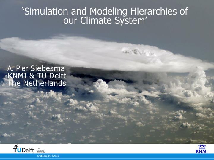
‘Simulation and Modeling Hierarchies of our Climate System’. A. Pier Siebesma KNMI & TU Delft The Netherlands. Uncertainties in Future Climate model Predictions. IPCC 2007. 2.5-4.3°C. 1900. Past. Future. Present. Earth’s Global Energy Balance. 342 W/m 2. Incoming solar radiation.

E N D
‘Simulation and Modeling Hierarchies of our Climate System’ A. Pier Siebesma KNMI & TU Delft The Netherlands
Uncertainties in Future Climate model Predictions IPCC 2007 2.5-4.3°C 1900 Past Future Present
Earth’s Global Energy Balance 342 W/m2 Incoming solar radiation 235 W/m2 107 W/m2 Outgoing long wave radiation Reflected solar radiation Temperature
Increase of Greenhouse Gases……. 342 W/m2 Incoming solar radiation …..decrease in outgoing long wave radiation 107 W/m2 Reflected solar radiation ….increase of temperature
……restored new Equilibrium 342 W/m2 Incoming solar radiation 235 W/m2 107 W/m2 Outgoing long wave radiation Reflected solar radiation Higher equilibrium temperature
If climate would be static………… Top of the atmosphere :Planetary Albedo R: net radiation at the TOA External Perturbation Zero feedback gain
If climate would be static………… Top of the atmosphere :Planetary Albedo R: net radiation at the TOA Planck Parameter Forcing for 2XCO2 External Perturbation Zero feedback gain Direct Warming
Dynamical Climate Model Feedbacks perturbation zero feedback gain feedback processes
Cloud feedback Surface albedo feedback Water vapor feedback Radiative effects only 2XCO2 Scenario for 12 Climate Models Dufresne & Bony, Journal of Climate 2008 Cloud effects “remain the largest source of uncertainty” in model based estimates of climate sensitivity IPCC 2007
Primarily due to marine low clouds Stratocumulus “Marine boundary layer clouds are at the heart of tropical cloud feedback uncertainties in climate models” (duFresne&Bony 2005 GRL) Shallow cumulus
1. The planetary scale Cloud cluster scale How did I get here? ~107 m ~105 m Cloud microphysical scale Cloud scale ~103 m ~10-6m - 1m
No single model can encompass all relevant processes mm 10 m 100 m 1 km 10 km 100 km 1000 km 10000 km Cloud microphysics turbulence Cumulus clouds Cumulonimbus clouds Mesoscale Convective systems Extratropical Cyclones Planetary waves DNS Subgrid Large Eddy Simulation (LES) Model Cloud System Resolving Model (CSRM) Numerical Weather Prediction (NWP) Model Global Climate Model
turbulence Resolved Scales convection clouds radiation ~ 100 km Small scales Large scales Schematic View of how scales are connected in traditional GCM’s Depiction of the interaction between resolved and parameterized unresolved cloud-related processes (convection, turbulence, clouds and radiation) in present-day climate models. (from Siebesma et al, Perturbed Clouds in our climate system MIT) Which are the problems, errors and uncertainties that we have to face with this approach?
1. Inherent lack of understanding of certain physical processes [100,600mm] < 100 mm >800mm • Uncertainties in ice and mixed phase microphysics: • Supersaturation • Liquid vs ice • Habits • Size distribution • Sedimentation • Interaction with radiation No fundamental equations available describing these properties and processes. Source : Andrew Heymsfield
ql=1 g/kg ql=0 2. Non-linear character of many cloud related processes Example 1: Autoconversion of cloud water to precipitation in warm clouds : Kessler Autoconversion Rate (Kessler 1969) With: ql : cloud liquid water ql : critical threshold H : Heaviside function A : Autoconversion rate GCM grid box Autoconversion rate is a convex function: Subgrid variabilityof liquid water needs to be known in order to estimate the autoconversion………. Larson et al. JAS 2001
qsat(T) . (T,qt) qt qt qsat T Example 2: Cloud fraction and Cloud liquid water Cloud fraction: Cloud liquid water: Subgrid variability of temperature and humidity needs to be known in order to estimate the grid box cloud fraction ac and liquid water content ql
x x Liquid water path (LWP) Example 3: Cloud Albedo Bias Plane parallel cloud Scu Cloud albedo a a(LWP) < a(LWP) Neglecting Cloud inhomogeneity causes a positive bias in the cloud albedo.
These biased errors slowly go away when increasing model resolution: • Typically allowed if x < 100m • So for all models operating at a coarser resolution additional information about the underlying Probability Density Function (pdf) is required of temperature, humidity (and vertical velocity). For Example: So if only….. we would know the pdf .
turbulence Resolved Scales convection clouds radiation ~ 250 km Small scales Large scales 3. Interactions between the various subgrid processes • Subgrid processes strongly interact with each other while in (most) GCM’s they only interact indirectly through the mean state leading to inconsistencies and biases.
4. Statistical versus Stochastic Convection • Traditionally (convection) parameterizations are deterministic: • Instantaneous grid-scale flow and mean state is taken as input and convective response is deterministic • One to one correspondency between sub-grid state and resolved state assumed. • Conceptually assumes that spatial average is a good proxy for the ensemble mean. ~500km e.g. subgrid cloud fraction :
4. Statistical versus Stochastic Convection Stochastic Convection That takes into account fluctuations so that the ensemble mean is not satisfied each timestep but more in a canonical sense Statistical ensemble mean Deterministic convection parameterization Microcanonical limit Convection Explicitly resolved 1km 100m 100km 1000km resolution
turbulence convection clouds radiation Resolved Scales 3.5 km Pathway 1: Global Cloud Resolving Modelling (Brute Force) NICAM simulation: MJO DEC2006 Experiment 3.5km run: 7 days from 25 Dec 2006 • Short timeslices • Testbed for interactions: • deep convection and the large scale • Boundary clouds, turbulence, radiation still unresolved MTSAT-1R NICAM 3.5km Miura et al. (2007, Science)
Resolved Scales (b) turbulence 2D CRM convection 5 km 250 km clouds radiation Pathway 2: Superparameterization
Pathway 2: Superparameterization What do we get? • Explicit deep convection • Explicit fractional cloudiness • Explicit cloud overlap and possible 3d cloud effects • Convectively generated gravity waves But….. A GCM using a super-parameterization is 2 to 3 orders of magnitude more expensive than a GCM that uses conventional parameterizations. On the other hand super-parameterizations provide a way to utilize more processors for a given GCM resolution Boundary Layer Clouds, Microphysics and Turbulence still needs to be parameterized
Pathway 3: Consistent based parameterizations Remarks: turbulence Resolved Scales convection Resolved Scales clouds radiation Large scales Unresolved scales ~100 km Increase consistency between the parameterizations! How? Topic of the coming week.
Use the full range of observations and simulation hierarchy.... GEWEX Cloud Systems Study (GCSS) Strategy. Climate Models NWP Models Single Column Models Large Eddy Simulation Direct Numerical Simulation Global Observational Data sets Field Campaigns Instrumented Sites
Global Climate Simulations Large Eddy Simulations Satellite data Laboratory experiments Direct Numerical Simulation Simulations Atmospheric Profiling stations Field campaigns Observations High Low resolution Scale Hierarchy
Example: Bulk Model (“parameterization”) of Scu topped PBL Minimal Mixed layer Model qt ql weDqt,i weDql,i zi VDql,0 VDqt,0 Plus closure:
Global Climate Simulations Large Eddy Simulations Satellite data Laboratory experiments high microphysical models Level of “understanding” or conceptualisation Mixed layer models Models/Parameterizations Direct Numerical Simulation Simulations low Atmospheric Profiling stations Field campaigns Observations High Low resolution Scale Hierarchy
Global Climate Simulations Large Eddy Simulations Satellite data Laboratory experiments high Conceptual models Statistical Mechanics Self-Organised Criticality Interface & microphysical models Level of “understanding” or conceptualisation Mixed layer models Models/Parameterizations Direct Numerical Simulation Simulations low Atmospheric Profiling stations Field campaigns Observations High Low resolution Scale Hierarchy
Complexity Dielectric Breakdown P.W. Anderson “More is Different”, Science 1977 “the emerge of collective properties with a large number of interacting elements” Galaxy distribution • Interacting elements: • Atoms in Physics • Macromolecules in Biology • People in economics • Convective cloud elements in atmospheric Science? Internet structure
Toy Example: Percolation p=probability of having a conductive bond 1-p = probability of having a insulating bond Phase Transitions in Statistical Mechanics p=0.3 pc=0.5 p=0.8 insulating conducting Transition point At the transistion point: scaling laws, fractal geometry, renormalization group theory But……This exotic behaviour is only achieved if the order parameter (p) is exactly set to the critical point.
Self Organized Criticality • In many non-equilibrium systems self-similarity and fractal behaviour emerges spontaneously (including atmosperic turbulence, convection and clouds) • Toy model that displays this features: Sand Pile Model. Add randomly grains of sand: Redistribute grains if a local threshold slope is reached: Causing avalanches of any scale (power law).
Global Climate Simulations Large Eddy Simulations Satellite data Laboratory experiments high Conceptual models Statistical Mechanics Self-Organised Criticality Interface & microphysical models Level of “understanding” or conceptualisation Mixed layer models Models/Parameterizations Direct Numerical Simulation Simulations low Atmospheric Profiling stations Field campaigns Observations High Low resolution Scale Hierarchy