Data Analysis: Descriptive Statistics

1. Data Analysis: Descriptive Statistics

2. “The government is very keen on amassing statistics. They will collect them, raise them to the nth power, take the cube root, and prepare wonderful diagrams. But you must never forget that every one of these figures comes in the first instance from the village watchman, who just puts down what he pleases.” Sir Josiah Stamp Commissioner of Inland Revenue (1896-1919)

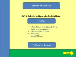
3. Statistics • Science of collecting, describing and interpreting data • Types • Descriptive • Inferential

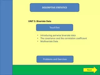
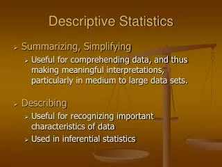
4. Techniques that allow you to organize and summarize data. Examples include graphs, percentages and averages Includes the collection, presentation and description of sample data Descriptive statistics come in a form of charts, tables and graphs Descriptive Statistics

5. Inferential • Techniques that allow you to offer conclusions about your data • Use sampling techniques, experimental designs, and statistical tests to make inferences about your data • Use observations: • Generalize from the sample to the population • Perform hypothesis testing • Determine relationships among variables • Make predictions • Inferential statistics allow to infer properties of an entire group (population) of individuals from a small number of those individuals (sample)

6. Definitions • Response variable • A characteristic of interest about each individual element of a population or sample • This is the characteristic being measured. If you want the income of all teachers in Mankato, your variable is income • Data • The set of values collected for the variable from each of the elements belonging to the sample. We could ask 10 teachers (our sample) their income (variable) and the 10 responses would be our data

7. Scales of measurement • Nominal data (naming data) • Classifies data into mutually exclusive (non overlapping) exhausting categories in which no order or rank can be imposed on the data • No logical ordering of categories • Categories are qualitative in nature • Examples: gender; religion; eye color; marital status

8. Cont’d • Ordinal (rank order data) • Classify data into categories that can be ranked, however precise differences between ranks don’t exist • Differences in amount of measured characteristic are discernible and numbers are assigned according to that amount • Properties of ordinal data: • Data are mutually exclusive • Data categories have some logical order • E.g. Results of a 400m race: 1st , 2nd, 3rd

9. Cont’d • Discrete Data • A quantitative variable whose set of possible values is countable • Consist of data that are whole numbers and have no decimal places • Often thought as counting data • Number of people in a lecture theatre • Number of lecture halls on MSU campus • Number of people who agree with a particular statement

10. Cont’d • Continuous Data • A variable that can take any real number • Height • Weight • Income

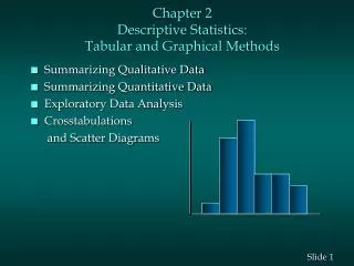
11. Organizing and Displaying data • The purpose of displaying data using graphics is to summarize raw data into an easy to read and presentable form. • From such graphs conclusions about the data can often be drawn without further analysis • Graphic presentation • Qualitative data • Bar Chart • Pie chart • Quantitative data • Frequency distribution and histogram

12. Bar Chart

13. Cont’d

14. Cont’d

15. Pie chart

16. Frequency distribution • A listing that pairs each value of a variable with its frequency • They can be classified into two types: • Ungrouped • Each value of variable in the distribution stands alone • Grouped • A set of classes are assigned

17. Ungrouped • Ungrouped because for each value of x (0 to 5) we have the number of times (f—its frequency) that appears in the data

18. Grouped

19. Cont’d • When constructing grouped frequency distributions, the following points should be borne in mind • Each class should be of the same width • The classes should be exclusive and exhaustive • Open-ended classes should be avoided • The number of classes should ideally be between 5 and 15 • To graph grouped frequency distributions we often use histograms • The bars of a histogram should touch as they represent the area of the same sample

20. Cont’d

21. Cont’d • Relative frequency • Frequency/total frequency • Cumulative frequency • Sum of the frequency of the class intervals as you go down each interval

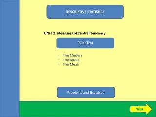
22. Measures of Central Tendency • The most commonly used characteristic of a set of data is its center or the point about which many of the observations are clustered • There are many different ways of measuring central tendency: • Mean • Median • Mode • Range

23. Mean • The arithmetic mean (or the average or simply mean) is computed by summing all numbers and dividing by the number of observations • The mean uses all the observations and each observation affects the mean

24. Median • The median is the middle value in an ordered array of observations • If there is an even number of data in the array, the median is the average of the two middle numbers • If there is an odd number of data in the array, the median is the middle number • For example, suppose you want to find the median for the following set of data: • 74, 66, 69, 68, 73, 70 • First we arrange the data in an ordered array: • 66, 68, 69, 73, 70, 74

25. Cont’d • Since there is an even number of data, the average of the middle two numbers (i.e. 69 and 73) is the median (142/2=71) • Generally the median provides a better measure of location than the mean when there are extremely large or small observations (i.e., when the data are skewed to the right or to the left • If the median is less than the mean, the data set is skewed to the right • If the median is greater than the mean, the data is skewed to the left

27. Mode • The mode is the most is the most frequent occurring value in a set of observation • Put simply, it is the most frequently occurring data value • For example, given 2, 3, 4, 5, 4, the mode is 4 because there are more fours than any other number—unimodal • Data may have two modes—bimodal • Observations with more than two modes are referred to as multimodal

28. Range • The range is the simplest measure of dispersion • The range can be thought in two ways: • As a quantity: the difference between the highest and lowest scores in a distribution • As an interval: the lowest and highest scores may be reported as the range

29. Cont’d

30. Cont’d • Range for sample 1: Either (97, 103) or 6 • Range for sample 2: Either (49, 151) or 102 • Range for Sample 3: Either (1, 199) or 198 • Each sample is clearly different from one another in terms the way the data is spread • The range is susceptible to extreme values; it only uses two values in your data for calculation

31. Cont’d • The range does not include all of the observations • Only the two most extreme values are included and these two numbers may be untypical observations

32. Quartiles • Quartiles divide the sorted data into quarters. Hence, for the first quartile (Q1) 25% of the data is below it and 75% above it • The second quartile (Q2-this is also the median) has 50% of the data below it and 50% above it • Finally, 75% of the observations are below Q3 while 25% are above

33. Calculating IQR • Inter quartile range (IQR) • Upper quartile minus the lower quartile • Sort (rank) the data and find the median (which is the middle value—the 50% position) • This effectively splits your data into two groups—below median and above median • Next we simply find the median of these two groups—this gives us the value at the 25% position and the 75% position

34. Cont’d

35. Cont’d • IQ range for sample 1: • The median is the 4th largest observation which is 100 • There are three data points below our median (97, 98, 99) • The median of these values is 98 • There are three data points above our median (101, 102, 103) • The median of these values is 102 • Hence, our IQ range is 102-98=4

36. Variance • Variance is the average of the squared deviations from the arithmetic mean • The following steps are used to calculate the variance • Find the arithmetic mean • Find the difference between each observation from the mean • Square these differences • Sum the square differences • Since the data is a sample, divide the number (from step 4 above) by the number of observations minus one.