Download
1 / 22
220 likes | 366 Views
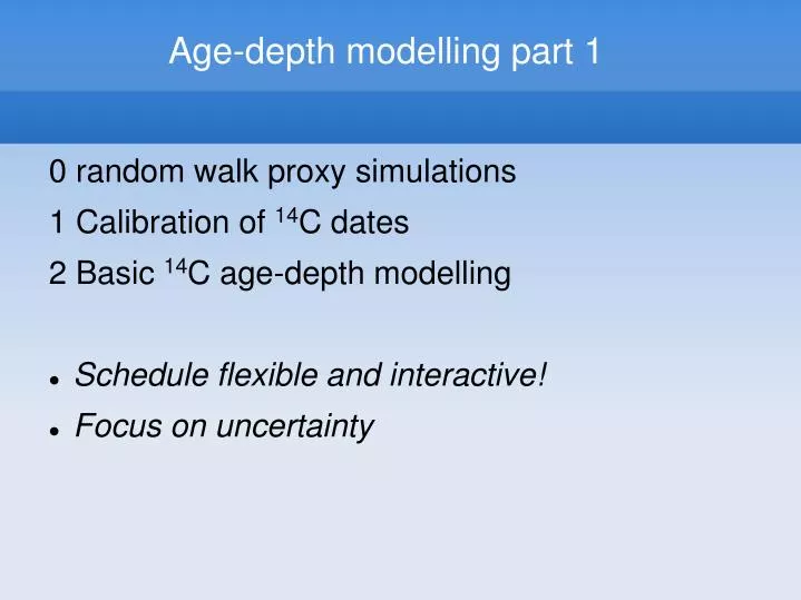
Age-depth modelling part 1. 0 random walk proxy simulations 1 Calibration of 14 C dates 2 Basic 14 C age-depth modelling Schedule flexible and interactive! Focus on uncertainty. R. Stats and graphing software Many user-provided modules Free, open-source Open R and type:

E N D
Age-depth modelling part 1 0 random walk proxy simulations 1 Calibration of 14C dates 2 Basic 14C age-depth modelling • Schedule flexible and interactive! • Focus on uncertainty
R Stats and graphing software Many user-provided modules Free, open-source Open R and type: plot(1:10, 11:20) x <- 1:10 ; y <- 11:20 ; plot(x, y, type='l') Case sensitive Previous commands: use up cursor
Random walk simulations Checkhttp://chrono.qub.ac.uk/blaauw/Random.R in browser Open R and load the link: Source ( url( 'http://chrono.qub.ac.uk/blaauw/Random.R' ) ) RandomEnv() RandomEnv(nforc=2, nprox=5) RandomProx()
Introduction – 14C decay • Atm. 12C (99%), 13C (1%), 14C (10-12) • 14C decays exponentially with time • Cease metabolism -> clock starts ticking • Measure ratio 14C/C to estimate age fossil
Calibrate – 14C age errors • Counting uncertainty AMS • Counting time (normal vs high-precision dates) • Sample size (larger = more 14C atoms) • Drift machine (need to correct, standards) • Preparation samples • Pretreatment, chemical & graphitisation • Material-dependent (e.g. trees, bone, coral) • Lab-specific • Every measurement will be bit different • Errors assumed to have Normal distribution
An alternative to the normal model • Christen and Perez 2009, Radiocarbon • Spread of dates often beyond expected • Reported errors are estimates • Propose an error multiplier, gamma • Results in t student distribution • No need for outlier modelling?
Calibrate - methods • Probability preferred over intercept • Less sensible to small changes in mean • Resulting cal.ranges make more sense • Procedure probability method: • What is prob. of cal.year x, given the date? • Calculate this prob. for all cal.ages Combine errors date and cal.curve √(2+sd2)
Calibrate - methods • Multimodal distributions • Which of the peaks most likely (Calib %)? • How report date? • 1 or 2 sd • sd range • mean±sd • mode • weighted mean (Telford et al. ‘05 Holocene) • why not plot the entire distribution!
Calibration, the equations • Calibration curve provides 14C ages µ for calendar years θ, µ(θ) • 14C measurement y ~ N(mean, sd) • Calibrate: find probability of y for θ N( µ(θ) , σ ), where σ2 = sd2 + σ(θ)2 for sufficiently wide range of θ
Calibrate - DIY • A) Using eyes/hands on handout paper • Imagine invisible arbitrary second axes for probs • Try to avoid using intercept • Try “cosmic schwung”, not mm precision • Don’t go from C14 to calBP! What is prob x cal BP? • Calibrated ranges?
1. clam ... R • R works in “workspace” • Remember where you work(ed)! • Change working dir via File > Change Dir • Or permanently using Desktop Icon (right-click, properties, start in) • Change R to your Clam workspace
1. Calibrating DIY • Define years: yr <- 1:1000 • A date: y <- 230; sdev <- 70 • Prob. for each yr: prob < - dnorm(yr, y, sdev) • plot(yr, prob, type=‘l’) • But we should calibrate: cc <- read.table(“IntCal09.14C”, header=TRUE) • cc[1:10,] • prob <- dnorm(cc[,2], y, sqrt(sdev^2+cc[,3]^2)) • plot(cc[,1], prob, type='l', xlim=c(0, 1000) )
Calibrate - DIY • clam (Blaauw, in press Quat Geochr) • Open R (via desktop icon or Start menu) • Change working directory to clam dir • Type: source(''clam.R'') [enter] • Type: calibrate(130, 35)
2. clam, calibrating • Type calibrate() • This calibrated 14C date of 2450 +- 50 BP • Type calibrate(130, 30) • Type calibrate(130, 30, sdev=1) • Try calibrating other dates, e.g., old ones • All clam code is open source, you can read the code to see/follow what it does
Feedback please • What was for you the best way to understand 14C calibration? Why? • Dedicated software (OxCal, Calib, clam) • Draw by hand • Animations • Equations