Download
1 / 60
600 likes | 797 Views
DNT 1013 DATA COMMUNICATIONS ------------------------------------------ CHAPTER 4: NETWORK LAYER. Prepared By: Mdm Noor Suhana Bt Sulaiman FKMT-NT, TATiUC. NETWORK LAYER: LOGICAL ADDRESSING. OSI Layers – Network Layer. The Network Layer

E N D
DNT 1013 DATA COMMUNICATIONS ------------------------------------------ CHAPTER 4: NETWORK LAYER Prepared By: Mdm Noor Suhana Bt Sulaiman FKMT-NT, TATiUC
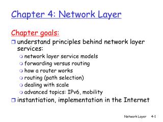
NETWORK LAYER: LOGICAL ADDRESSING
OSI Layers – Network Layer The Network Layer • Performs network routing, flow control, segmentation, and error control functions • The router operates at this layer • Uses local addressing scheme • Example – IP, token ring
Network Layer • Concerned with getting packets from source to destination. • The network layer must know the topology of the subnet and choose appropriate paths through it. • When source and destination are in different networks, the network layer (IP) must deal with these differences. • Key issue: what service does the network layer provide to the transport layer(connection-oriented or connectionless).
Network Layer Design Goals • The services provided by the network layer should be independent of the subnet topology. • The Transport Layer should be shielded from the number, type and topology of the subnets present. • The network addresses available to the Transport Layer should use a uniform numbering plan (even across LANs and WANs).
Messages Messages Segments Transport layer Transport layer Network service Network service Network layer Network layer Network layer Network layer End system b End system a Data link layer Data link layer Data link layer Data link layer Physical layer Physical layer Physical layer Physical layer
Machine B Machine A Application Application Transport Transport Router/Gateway Internet Internet Internet Network Interface Network Interface Network Interface Network 1 Network 2
Datagram Packet Switching Packet 1 Packet 1 Packet 2 Packet 2 Packet 2
Routing Table in Datagram Network Output port Destination address 0785 7 1345 12 1566 6 2458 12
Orientation • IP (Internet Protocol) is a Network Layer Protocol. • IP’s current version is Version 4 (IPv4). It is specified in RFC 891.
Application protocol • IP is the highest layer protocol which is implemented at both routers and hosts
IP Service • Delivery service of IP is minimal • IP provide provides an unreliable connectionless best effort service (also called: “datagram service”). • Unreliable: IP does not make an attempt to recover lost packets • Connectionless:Each packet (“datagram”) is handled independently. IP is not aware that packets between hosts may be sent in a logical sequence • Best effort: IP does not make guarantees on the service (no throughput guarantee, no delay guarantee,…) • Consequences: • Higher layer protocols have to deal with losses or with duplicate packets • Packets may be delivered out-of-sequence
IP Service • IP supports the following services: • one-to-one (unicast) • one-to-all (broadcast) • one-to-several (multicast) • IP multicast also supports a many-to-many service. • IP multicast requires support of other protocols (IGMP, multicast routing) unicast broadcast multicast
NETWORK LAYER: ADDRESS MAPPING, ERROR REPORTING & MULTICASTING
Address Mapping • The delivery of a packet to a host or a router requires two levels of addressing: logical and physical. • We need to be able to map a logical address to its corresponding physical address and vice versa. • This can be done by using either static or dynamic mapping.
DHCP provides static and dynamic address allocation that can bemanual or automatic.
ICMP • The IP protocol has no error-reporting or error-correcting mechanism. • The IP protocol also lacks a mechanism for host and management queries. • The Internet Control Message Protocol (ICMP) has been designed to compensate for the above two deficiencies. • It is a companion to the IP protocol
Important points about ICMP error messages: ❏ No ICMP error message will be generated in response to a datagram carrying an ICMP error message. ❏ No ICMP error message will be generated for a fragmented datagram that is not the first fragment. ❏ No ICMP error message will be generated for a datagram having a multicast address. ❏ No ICMP error message will be generated for a datagram having a special address such as 127.0.0.0 or 0.0.0.0.
Example 21.3 We use the ping program to test the server fhda.edu. The result is shown on the next slide. The ping program sends messages with sequence numbers starting from 0. For each probe it gives us the RTT time. The TTL (time to live) field in the IP datagram that encapsulates an ICMP message has been set to 62. At the beginning, ping defines the number of data bytes as 56 and the total number of bytes as 84. It is obvious that if we add 8 bytes of ICMP header and 20 bytes of IP header to 56, the result is 84. However, note that in each probe ping defines the number of bytes as 64. This is the total number of bytes in the ICMP packet (56 + 8).
We use the traceroute program to find the route from the computer voyager.deanza.edu to the server fhda.edu. The following shows the result: The unnumbered line after the command shows that the destination is 153.18.8.1. The packet contains 38 bytes: 20 bytes of IP header, 8 bytes of UDP header, and 10 bytes of application data. The application data are used by traceroute to keep track of the packets.
ICMPv6 • Another protocol that has been modified in version 6 of the TCP/IP protocol suite is ICMP (ICMPv6). • This new version follows the same strategy and purposes of version 4.
Figure 21.11 Comparison of network layer between IPv4 and IPv6
Table 21.3 Comparison of error-reporting messages in ICMPv4 and ICMPv6
Table 21.4 Comparison of query messages in ICMPv4 and ICMPv6
IP Address • An IP address is a unique number that is used to identify a network device. • An IP address is represented as a 32-bit binary number, divided into four octets (groups of eight bits): • Example: 10111110.01100100.00000101.00110110 • An IP address is also represented in a dotteddecimal format. • Example: 190.100.5.54 • When a host is configured with an IP address, it is entered as a dotted decimal number, such as 192.168.1.5. • Unique IP addresses on a network ensure that data can be sent to and received from the correct network device.
IP Address Classes • Class A • Large networks, implemented by large companies and some countries • Class B • Medium-sized networks, implemented by universities • Class C • Small networks, implemented by ISP for customer subscriptions • Class D • Special use for multicasting • Class E • Used for experimental testing
An Ethernet multicast physical address is in the range 01:00:5E:00:00:00 to 01:00:5E:7F:FF:FF.
Example 21.9 We use netstat (see next slide) with three options: -n, -r, and -a. The -n option gives the numeric versions of IP addresses, the -r option gives the routing table, and the -a option gives all addresses (unicast and multicast). Note that we show only the fields relative to our discussion. “Gateway” defines the router, “Iface” defines the interface. Note that the multicast address is shown in color. Any packet with a multicast address from 224.0.0.0 to 239.255.255.255 is masked and delivered to the Ethernet interface.
NETWORK LAYER: DELIVERY, FORWARDING & ROUTING
Routing • Routing algorithm:: that part of the Network Layer responsible for deciding on which output line to transmit an incoming packet. • Remember: For virtual circuit subnets the routing decision is made ONLY at set up. • Algorithm properties:: correctness, simplicity, robustness, stability, fairness, optimality, and scalability.
Adaptive Routing based on current measurements of traffic and/or topology. 1. centralized 2. isolated 3. distributed Non-Adaptive Routing flooding static routing using shortest path algorithms Routing Classification
Shortest Path Routing • Bellman-Ford Algorithm [Distance Vector] • Dijkstra’s Algorithm [Link State] What does it mean to be the shortest (or optimal) route? • Minimize mean packet delay • Maximize the network throughput • Mininize the number of hops along the path
Internetwork Routing[Halsall] Adaptive Routing Centralized Distributed [RCC] [IGP] [EGP] Intradomain routing Interdomain routing [BGP,IDRP] Interior Gateway Protocols Exterior Gateway Protocols Distance Vector routing Link State routing [RIP] [OSPF,IS-IS,PNNI]
Distance Vector Routing • Historically known as the old ARPANET routing algorithm {or known as Bellman-Ford algorithm}. • Basic idea: each network node maintains a Distance Vector table containing the distance between itself and ALL possible destination nodes. • Distances are based on a chosen metric and are computed using information from the neighbors’ distance vectors. • Metric: usually hops or delay