Propagation Directions and Kinematics of the Coronal Mass Ejections of August 2010

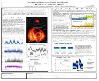
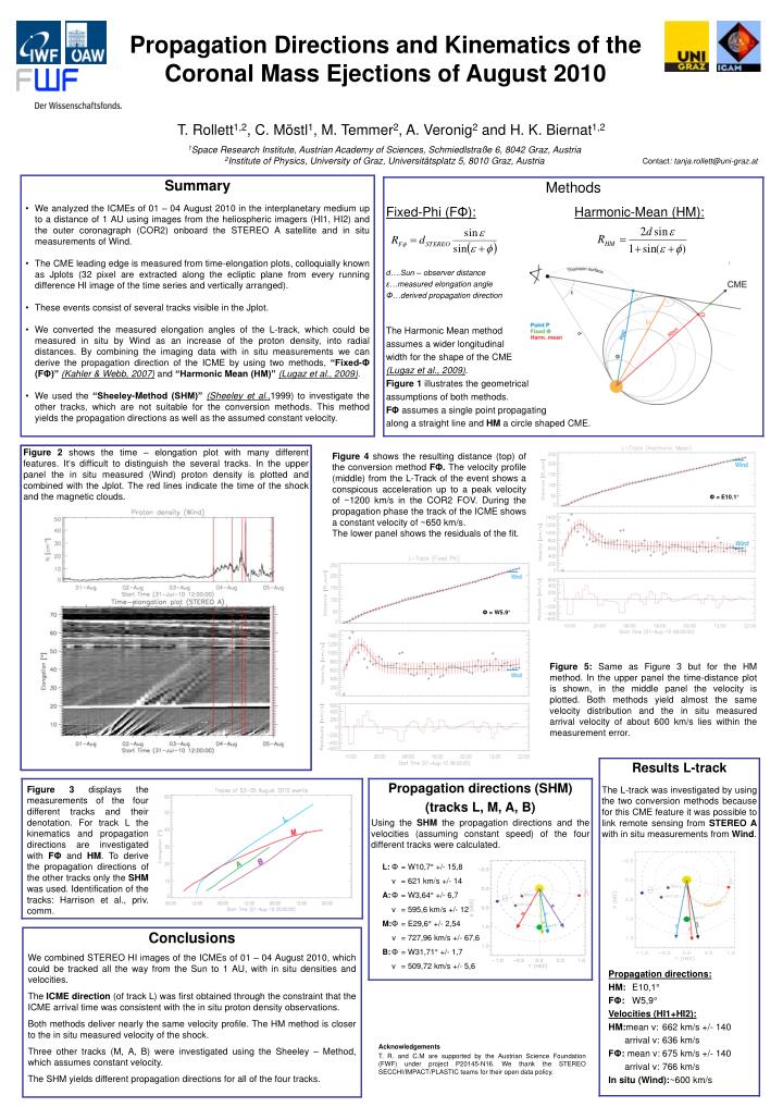
1. Propagation Directions and Kinematics of the Coronal Mass Ejections of August 2010 T. Rollett1,2, C. Möstl1, M. Temmer2, A. Veronig2 and H. K. Biernat1,2 1Space Research Institute, Austrian Academy of Sciences, Schmiedlstraße 6, 8042 Graz, Austria 2Institute of Physics, University of Graz, Universitätsplatz 5, 8010 Graz, Austria Contact: tanja.rollett@uni-graz.at • Summary • We analyzed the ICMEs of 01 – 04 August 2010 in the interplanetary medium up to a distance of 1 AU using images from the heliospheric imagers (HI1, HI2) and the outer coronagraph (COR2) onboard the STEREO A satellite and in situ measurements of Wind. • The CME leading edge is measured from time-elongation plots, colloquially known as Jplots (32 pixel are extracted along the ecliptic plane from every running difference HI image of the time series and vertically arranged). • These events consist of several tracks visible in the Jplot. • We converted the measured elongation angles of the L-track, which could be measured in situ by Wind as an increase of the proton density, into radial distances. By combining the imaging data with in situ measurements we can derive the propagation direction of the ICME by using two methods, “Fixed-Φ (FΦ)”(Kahler & Webb, 2007) and “Harmonic Mean (HM)”(Lugaz et al., 2009). • We used the “Sheeley-Method (SHM)”(Sheeley et al.,1999) to investigate the other tracks, which are not suitable for the conversion methods.This method yields the propagation directions as well as the assumed constant velocity. Figure 2 shows the time – elongation plot with many different features. It‘s difficult to distinguish the several tracks. In the upper panel the in situ measured (Wind) proton density is plotted and combined with the Jplot. The red lines indicate the time of the shock and the magnetic clouds. Figure 4 shows the resulting distance (top) of the conversion method FΦ. The velocity profile (middle) from the L-Track of the event shows a conspicous acceleration up to a peak velocity of ~1200 km/s in the COR2 FOV. During the propagation phase the track of the ICME shows a constant velocity of ~650 km/s. The lower panel shows the residuals of the fit. Φ = E10.1° Φ = W5.9° Figure 5: Same as Figure 3 but for the HM method. In the upper panel the time-distance plot is shown, in the middle panel the velocity is plotted. Both methods yield almost the same velocity distribution and the in situ measured arrival velocity of about 600 km/s lies within the measurement error. Figure 3 displays the measurements of the four different tracks and their denotation. For track L the kinematics and propagation directions are investigated with FΦ and HM. To derive the propagation directions of the other tracks only the SHM was used. Identification of the tracks: Harrison et al., priv. comm. L:Φ = W10,7° +/- 15,8 v = 621 km/s +/- 14 A:Φ = W3,64° +/- 6,7 v = 595,6 km/s +/- 12 M:Φ = E29,6° +/- 2,54 v = 727,96 km/s +/- 67,6 B:Φ = W31,71° +/- 1,7 v = 509,72 km/s +/- 5,6 Conclusions We combined STEREO HI images of the ICMEs of 01 – 04 August 2010, which could be tracked all the way from the Sun to 1 AU, with in situ densities and velocities. The ICME direction (of track L) was first obtained through the constraint that the ICME arrival time was consistent with the in situ proton density observations. Both methods deliver nearly the same velocity profile. The HM method is closer to the in situ measured velocity of the shock. Three other tracks (M, A, B) were investigated using the Sheeley – Method, which assumes constant velocity. The SHM yields different propagation directions for all of the four tracks.