Download
1 / 16
160 likes | 247 Views
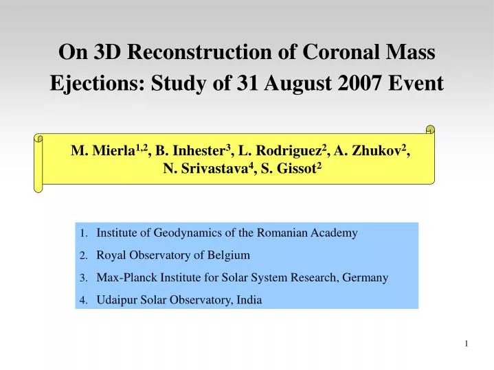
On 3D Reconstruction of Coronal Mass Ejections: Study of 31 August 2007 Event. M. Mierla 1,2 , B. Inhester 3 , L. Rodriguez 2 , A. Zhukov 2 , N. Srivastava 4 , S. Gissot 2. Institute of Geodynamics of the Romanian Academy Royal Observatory of Belgium

E N D
On 3D Reconstruction of Coronal Mass Ejections: Study of 31 August 2007 Event M. Mierla1,2, B. Inhester3, L. Rodriguez2, A. Zhukov2, N. Srivastava4, S. Gissot2 Institute of Geodynamics of the Romanian Academy Royal Observatory of Belgium Max-Planck Institute for Solar System Research, Germany Udaipur Solar Observatory, India
Contents Introduction 31 August 2007 CME LCT + Triangulation Method – description – constraints Longitudinal Extension of the CME Summary
Introduction Since the launch of STEREO spacecraft in October 2006, several reconstruction techniques were successfully used to derive the direction of propagation and the true speed of coronal mass ejections (CMEs) at distances close to the Sun (coronagraphs fields of view - see the review by Mierla et al. 2010). • Attempts to reconstruct the CME 3D configuration (full geometric shape) have been done by: • Using forward modelling (e.g. Thernisien et al. 2009) (a priori known shape of the CME) • Polarized ratio method (Moran et al. 2010, Mierla et al. 2009) (weighted mean distance of the CME plasma density along each line of sight)
Introduction The aim of this study: Getting the full 3D geometry of a CME by using local correlation tracking method (to identify the same feature in STEREO/COR images) plus triangulation (to derive its 3D location). Constraints: 1) the complexity of the CMEs morphologies (bubble-like shapes, twisted flux-ropes etc.); 2) the correct identification of the same feature in the two images; 3) optically thin plasma.
31 August 2007 CME
Data pre-processing Co-align the images in STEREO mission plane: same Sun center, same pixel resolution they are rotated such that epipolar north is at the top of the image Inhester, 2006
Correlation Technique The correlation coefficient ρX,Y between two random variables X and Y with expected values μX and μY and standard deviations σX and σY is defined as: where E is the expected value operator and cov means covariance. The standard deviation is a measure of the dispersion of a collection of values: Covariance provides a measure of the strength of the correlation between two or more sets of random variates:
img B (Y) img A (X) Correlation Technique Note that the images are co-aligned in STEREO mission plane Program (Sam): bm_flow, imgA, imgB, neigh, lag_window, result_x, result_y, result ρX,Y< 0: anti-correlation; ρX,Y ~ 0: no correlated; ρX,Y > 0.9: high correlation = lag or search window (for e.g. 256 x 3 pixels) = area where correlation is calculated (for e.g 11 x 11 pixels)
Correlation – constraints 1. The technique finds high correlation coefficients for noisy data (low intensity or low signal-to-noise pixels). Solution: remove the noise How? Setting a threshold for each image. 2. For a smooth feature (along the epipolar line) the method finds more than a maxima in a search window Solution: take the point in the search window closest to the center of mass.
Tie-point reconstruction Inhester, 2006 use the program from solar soft (Bill): scc_measure.pro or depth_reconstruction.pro (Sam)
Longitudinal Extension of the CME COR2 (1 September 2007, 01:52 UT) COR1 (31 August 2007, 21:30 UT)
Mean value of all reconstructed points obtained from LCT-TP method, in HEEQ coordinate system.
Summary • The LCT-TP results show some scatter in the direction parallel to the line-of-sight. • The spread should indicate the depth extent of the CME, if the correlation maxima are due to identical plasma fluctuations inside the CME. • But, as it is a statistical approach some noise and scatter must be expected. • Unfortunately, we have no means to check what the real spread of the CME is. • We can check how good the LCT-TP method is by applying it to a model CME.