Download
1 / 67
690 likes | 910 Views
Applications of Genetic Algorithms to Resource-Constrained Scheduling Tasks. Keith Downing Dept. of Computer and Information Sciences The Norwegian University of Science & Technology Trondheim, Norway keithd@idi.ntnu.no. Outline. Introduction to Evolutionary Algorithms Basic Concepts

E N D
Applications of Genetic Algorithms to Resource-Constrained Scheduling Tasks Keith Downing Dept. of Computer and Information Sciences The Norwegian University of Science & Technology Trondheim, Norway keithd@idi.ntnu.no
Outline • Introduction to Evolutionary Algorithms • Basic Concepts • Simple Scheduling Example • Applying EA’s to Scheduling Problems • Travelling Salesman • Job Sequencing • Classic Job-Shop Scheduling * Main Focus: Representational Issues
Sex Recombination & Mutation Morphogenesis Darwinian Evolution Physiological, Behavioral Phenotypes Natural Selection Ptypes Reproduction Gtypes Genotypes Genetic
R &M Translate Recombination & Mutation Evolutionary Algorithms Semantic Parameters, Code, Neural Nets, Rules Performance Test P,C,N,R Generate Bits Bit Strings Syntactic
Next Generation Evolutionary Computation = Parallel Stochastic Search Biased Roulette Wheel 6 1 5 Selection Biasing 4 2 Translation & Performance Test 3 Selection Mutation Crossover
Types of Evolutionary Algorithms Genetic Algorithms (Holland, 1975) Representation: Bit Strings => Integer or real feature vectors Syntactic crossover (main) & mutation (secondary) Evolutionary Strategies (Recehenberg, 1972; Schwefel, 1995) Representation: Real-valued feature vectors Semantic mutation (main) & crossover (secondary) Evolutionary Programs (Fogel, Owens & Walsh, 1966; Fogel, 1995) Representation: Real-valued feature vectors or Finite State Machines Semantic mutation (only) View each individual as a whole species, hence no crossover Genetic Programs (Koza, 1992) Representation: Computer programs (typically in LISP) Syntactic crossover (main) & mutation (secondary)
0 1 1 1 0 1 0 0 1 0 1 1 1 0 0 0 1 1 1 1 1 0 0 1 0 0 0 0 1 1 1 1 0 1 0 1 1 0 1 1 1 0 1 0 1 0 0 1 0 1 7 P1 7 P2 14 4 15 5 X 11 2 P3 11 2 Evolutionary Computation Requirements • Domain that supports quantitative fitness assignment • Fitness function that accurately evaluates performance • Representation for solutions that tolerates mutation & crossover Classic Genetic Algorithm
Using Evolutionary Algorithms When • Large, rough search spaces • Satisficing or Optimization problems • Entire solutions are easily generated and tested • Exhaustive search methods are too slow • Heuristic search methods cannot find good solutions (e.g. Stuck at local max) How • Determine EA-amenable representation of solutions • Define fitness function • Define selection function = roulette-wheel biasing function (f: fitness -> area) • Set key EA parameters: population size, mutation rate, crossover rate, # generations, etc. * EA’s are easy to write, and there’s lots of freeware! * Specific problems often require specific representations & genetic operators
Application Areas for Evolutionary Algorithms • Optimization: Controllers, Job Schedules, Networks(TSP) • Electronics: Circuit Design (GP) • Finance: Stock time-series analysis & prediction • Economics: Emergence of Markets, Pricing & Purchasing Strategies • Sociology: cooperation, communication, ANTS! • Computer Science • Machine Learning: Classification, Prediction… • Algorithm design: Sorting networks • Biology • Immunology: natural & virtual (computer immune system) • Ecology: arms races, coevolution • Population genetics: roles of mutation, crossover & inversion • Evolution & Learning: Baldwin Effect, Lamarckism…
P5 P1 P7 P3 P0 P6 P4 P2 Process Scheduling (Kidwell, 1993) • Task pairs (run + communicate result) to be run on a set of processors • ((7, 16) (11, 22) (12, 40), (15, 22)….) • A task’s run must finish before result sending begins • All processors share a central communication line (bus) • Each processor can handle only one task at a time. • Each processor is capable of running any of the tasks • Only one processor at a time can send its message • A task cannot be removed from a processor until both run & send are finished • Tasks run on the main processor, P0, require no communication time, whereas tasks run on all other processors must send their message to P0 Goal: Schedule the tasks on processors so as to minimize the total timespan
Processor for Task #1 Processor for Task #4 ... ... (2 3 4 1 3 1 …….) 001000110100000100110001…. Process Schedule Optimization using the Genetic Algorithm Use GA to search the space of possible schedules (solutions) 1. Represent schedule in a GA-amenable form (i.e. linearize it) 2. Define a fitness function Fitness = MaxTimespan - Timespan * Lower timespan => Higher fitness Other possibilities: 1/(1 + (Timespan - MinTimespan))
GA-based Schedule Optimization *Compute schedule’s timespan by running on a process-network simulator. 1. Remove next task (whose assigned processor is open) from task-list and start simulating it on that processor. 2. Remove tasks from processors as soon as they finish running & sending 3. Define a biasing function to convert fitness to a proportion of the roulette wheel Sigma Scaling: (One of many standard biasing functions): ExpVal(x) = Max ( 0, 1 + (Fitness (x) - AvgFitness) / (2 * StDevFitness)) Normalizing: Roulette-Wheel%(x) = ExpVal(x) / SumofAllExpVals 4. Select Mutation and Crossover Rates: pmut = 0 .01; pcross = 0.75 5. Select a population size popsize = 10 6. Select # of generations: numgen = 10 7. Run the Genetic Algorithm Generates a random initial population (of schedules) and evolves them via sigma-scaling selection, crossover and mutation for numgen generations
Kidwell’s (1993) Task List ((7 16) (11 22) (12 40) (15 22) (17 23) (17 23) (19 23) (20 28) (20 27) (26 27) (28 31) (36 37) (31 29) (28 22) (23 19) (22 18) (22 17) (29 16) (27 16) (35 15)) MaxTime = Sum of all run & send times = 916 time units Use 8 processors: P0 - P7, with P0 being the master processor
Population of Schedules (Generation # 0) These are randomly-generated: Processor List 1: Span: 401 Fitn: 515 (11.0%)| (1 2 1 3 6 7 2 0 0 4 5 1 6 0 5 5 4 7 4 6) 2: Span: 383 Fitn: 533 (13.7%)| (1 0 1 0 0 4 0 1 0 5 3 6 2 5 5 5 1 3 5 7) 3: Span: 426 Fitn: 490 ( 7.1%)| (6 2 2 7 6 5 2 6 7 6 6 5 3 4 0 1 0 2 0 7) 4: Span: 415 Fitn: 501 ( 8.8%)| (5 0 5 7 1 2 5 4 2 6 3 6 2 0 0 4 1 7 3 1) 5: Span: 377 Fitn: 539 (14.7%)| (4 2 0 6 2 1 2 0 1 6 3 2 2 3 3 4 0 3 0 1) 6: Span: 435 Fitn: 481 ( 5.7%)| (3 2 7 7 6 0 3 1 4 7 7 5 1 0 4 6 5 5 5 6) 7: Span: 439 Fitn: 477 ( 5.1%)| (0 3 2 3 2 2 7 0 4 5 2 1 6 3 1 7 1 0 3 2) 8: Span: 410 Fitn: 506 ( 9.6%)| (2 5 2 1 0 0 2 2 5 0 1 3 6 1 3 3 4 6 2 0) 9: Span: 337 Fitn: 579 (20.9%)| (1 0 0 7 0 4 3 1 1 0 0 2 4 1 2 4 6 4 7 6) 10: Span: 449 Fitn: 467 ( 3.5%)| (2 2 2 4 1 4 4 6 6 4 7 4 0 6 2 5 2 7 7 7) Avg Fitness: 508.80 StDev Fitness: 32.28
Population of Schedules (Generation # 1) 1: Span: 366 Fitn: 550 (12.1%)| (1 0 0 3 0 4 2 1 0 1 3 6 4 5 7 4 5 7 5 6) 2: Span: 406 Fitn: 510 ( 7.9%)| (1 0 1 4 0 4 1 1 1 4 0 2 2 1 0 5 2 0 7 7) 3: Span: 377 Fitn: 539 (11.0%)| (4 2 0 6 2 1 2 0 1 6 3 2 2 3 3 4 0 3 0 1) 4: Span: 464 Fitn: 452 ( 1.8%)| (1 0 1 3 0 4 2 0 1 4 4 2 4 1 5 5 4 6 4 6) 5: Span: 366 Fitn: 550 (12.1%)| (1 2 0 7 6 7 3 1 0 0 1 1 6 0 2 4 6 5 7 6) 6: Span: 337 Fitn: 579 (15.2%)| (1 0 0 7 0 4 3 1 1 0 0 2 4 1 2 4 6 4 7 6) 7: Span: 337 Fitn: 579 (15.2%)| (1 0 0 7 0 4 3 1 1 0 0 2 4 1 2 4 6 4 7 6) 8: Span: 415 Fitn: 501 ( 7.0%)| (5 0 5 7 1 2 5 4 2 6 3 6 2 0 0 4 1 7 3 1) 9: Span: 465 Fitn: 451 ( 1.7%)| (5 5 7 7 1 2 5 2 3 6 1 6 2 1 0 5 1 7 2 1) 10: Span: 329 Fitn: 587 (16.0%)| (2 0 0 1 0 0 2 4 4 0 3 3 6 0 3 2 4 6 3 0) Avg Fitness: 529.80 StDev Fitness: 47.43
Population of Schedules (Generation # 2) 1: Span: 337 Fitn: 579 (11.7%)| (1 0 0 7 0 0 6 0 2 6 3 6 0 4 1 4 1 7 1 1) 2: Span: 465 Fitn: 451 ( 0.0%)| (5 0 5 3 1 6 1 5 0 1 3 6 6 1 6 4 5 7 7 6) 3: Span: 366 Fitn: 550 ( 8.8%)| (1 2 0 7 6 7 3 1 0 0 1 1 6 0 2 4 6 5 7 6) 4: Span: 329 Fitn: 587 (12.5%)| (2 0 0 1 0 0 2 4 4 0 3 3 6 0 3 2 4 6 3 0) 5: Span: 329 Fitn: 587 (12.5%)| (2 0 0 1 0 0 2 4 4 0 3 3 6 0 3 2 4 6 3 0) 6: Span: 270 Fitn: 646 (18.4%)| (1 0 0 5 0 0 2 0 0 0 3 3 4 0 2 2 4 6 3 2) 7: Span: 364 Fitn: 552 ( 9.0%)| (2 0 0 3 0 4 3 5 5 0 0 2 6 1 3 4 6 4 7 4) 8: Span: 337 Fitn: 579 (11.7%)| (1 0 0 7 0 4 3 1 1 0 0 2 4 1 2 4 6 4 7 6) 9: Span: 347 Fitn: 569 (10.7%)| (5 0 1 7 1 6 1 4 0 0 1 2 2 0 0 4 5 7 7 0) 10: Span: 410 Fitn: 506 ( 4.5%)| (1 0 4 7 0 0 7 1 3 6 2 6 4 1 2 4 2 4 3 7) Avg Fitness: 560.60 StDev Fitness: 49.61
Population of Schedules (Generation # 6) 1: Span: 263 Fitn: 653 (10.6%)| (1 0 0 7 0 4 6 0 0 4 3 7 0 0 0 0 5 6 3 6) 2: Span: 232 Fitn: 684 (16.7%)| (1 0 0 5 0 0 2 0 0 6 3 3 0 0 2 2 0 7 1 0) 3: Span: 325 Fitn: 591 ( 0.0%)| (1 0 0 5 0 0 6 0 0 2 3 3 4 0 3 4 5 7 3 2) 4: Span: 261 Fitn: 655 (11.0%)| (1 0 0 7 0 0 2 0 0 0 3 2 0 0 2 0 1 6 3 2) 5: Span: 249 Fitn: 667 (13.3%)| (1 0 0 5 0 0 2 0 0 2 3 6 0 0 3 0 5 6 3 2) 6: Span: 255 Fitn: 661 (12.1%)| (1 0 0 5 0 0 6 0 0 0 3 3 0 0 1 0 5 7 3 2) 7: Span: 292 Fitn: 624 ( 4.8%)| (1 0 0 7 0 0 3 0 0 0 3 3 4 0 0 4 1 6 3 2) 8: Span: 269 Fitn: 647 ( 9.4%)| (1 0 0 7 0 4 6 0 0 4 3 7 0 0 2 0 4 6 3 6) 9: Span: 247 Fitn: 669 (13.7%)| (1 0 0 5 0 0 2 0 0 0 3 7 4 0 0 4 1 6 3 2) 10: Span: 274 Fitn: 642 ( 8.4%)| (1 0 0 7 0 0 2 0 0 0 3 3 0 0 3 0 5 6 3 2) Avg Fitness: 649.30 StDev Fitness: 24.87
Population of Schedules (Generation # 9) 1: Span: 265 Fitn: 651 ( 0.4%)| (1 0 0 5 0 0 2 0 0 2 3 6 0 0 1 0 5 7 3 2) 2: Span: 241 Fitn: 675 (12.3%)| (1 0 0 7 0 0 2 0 0 4 3 3 0 0 3 0 0 6 1 0) 3: Span: 238 Fitn: 678 (13.8%)| (1 0 0 5 0 0 6 0 0 6 3 3 0 0 1 0 1 6 1 0) 4: Span: 258 Fitn: 658 ( 3.8%)| (1 0 0 5 0 0 6 0 0 6 3 2 0 0 0 0 0 7 1 0) 5: Span: 248 Fitn: 668 ( 8.8%)| (1 0 0 5 0 0 2 0 0 2 3 3 0 0 1 0 1 6 3 0) 6: Span: 246 Fitn: 670 ( 9.8%)| (1 0 0 5 0 0 6 0 0 6 3 7 0 0 1 0 5 7 1 2) 7: Span: 246 Fitn: 670 ( 9.8%)| (1 0 0 5 0 0 2 0 0 4 3 3 0 0 1 0 5 7 1 2) 8: Span: 242 Fitn: 674 (11.8%)| (1 0 0 5 0 0 6 0 0 2 3 6 0 0 3 0 1 6 3 0) 9: Span: 226 Fitn: 690 (19.7%)| (1 0 0 5 0 0 2 0 0 0 3 6 0 0 3 0 5 6 3 2) 10: Span: 246 Fitn: 670 ( 9.8%)| (5 0 0 5 0 0 2 0 0 2 3 6 0 0 3 0 5 7 3 2) Avg Fitness: 670.40 StDev Fitness: 10.06 (Convergence)
Process-Schedule Evolution GA falls off a peak Convergence
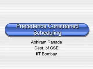
Travelling Salesman Problem (TSP) Given: N cities & matrix of distances between them. Find:Shortest cyclic tour that visits all cities. • NP-Hard: Exponential to both find solutions & to verify solutions • Heuristic Methods: Find optimal solutions when N< 1000. • Genetic Algorithm: Find good solutions for any N • Applications: Network building, Delivery routing, Sequence scheduling...
Applying GAs to TSP Fitness Function: 1/tour-length or optimal-tour-length/tour-length Chromosome: Direct Representation: List of cities (standard approach) 7 3 25 31 12 1 5 14…. Indirect Representation: List of next city to pull from ordered list and insert into the solution sequence 1 1 2 3 5…. => 1 2 4 6 9… Crossover Standard Bit or Integer Cross: Only works for indirect representations Location Preserving: Children inherit, as much as possible, cities in same gene location as parents Edge Preserving: Children inherit, as much as possible, city-city edges from parents (actual edge locations in the chromosome may vary from parent to kid) *Crossover is the key element to TSP GA’s - and where most research is done.
6 3 2 1 5 6 2 x 6; 0 x 4 6 3 2 5 4 1 4 2 3 1 5 6 X 4 2 3 5 4 1 2 x 4; 0 x 6 Representational Issues for GA-based TSP • Standard Crossover & Mutation are purely syntactic => pay no attention to semantics (i.e. The meanings of the bits or integers that they manipulate). • Direct representations often embody constraints that simple crossover & mutation cannot enforce. • Indirect representations usually involve fewer constraints, so simple crossover & mutation are often sufficient. • Compare to Process Scheduling (Kidwell), where constraints (i.e. All alleles between 0 and N) were easy to enforce.
Partially-Mapped Crossover (PMX) Goldberg (1985) 1. Choose equal-length segments to swap 2. Create a mapping between corresponding elems of the segments 3. Swap the segments 4. Apply the map to each child to restore completeness Select Segments P1: 1 6 3 4 5 7 2 8 P2: 3 7 6 5 8 1 2 4 Create Map (4 <=> 5; 5 <=> 8; 7<=> 1) Swap K1’: 1 635 8 1 28 Blue positions must be changed via mapping K2’: 3 7 6 4 5 7 2 4 Apply Map (twice for last position in this eg.) K1: 7 635 8 1 24 K2: 3 1 6 4 5 7 2 8
Subtour Operations (Cleveland & Smith, ‘89) Subtour Chunking • Select random chunks from the parents • Prune chunk of cities that already exist in the child • Insert chunk into child position as close as possible to its position in parent P1: (9 4 3)32(6 8 7 1)1(5 10)5 P2: 3 5 8 (7 10 4 6)2 9 (2 1)4 K1: 9 3 10 4 6 8 7 12 5 Subtour Replacement Find chunks with same elems in both parents and swap them P1: 1 5 6 3 2 4 8 7 P2: 2 7 4 8 1 6 5 3 K1: 1 5 6 3 2 7 4 8 K2: 24 8 71 6 5 3
Inheritance • For GA’s to make progress, they must pass on many of the good features from generation G to generation G+1. • Hence, when parents crossover, the good features of each should be preserved in at least one of the children. • Biology: Heritability = degree to which children resemble their parents (Xkid-avg - Xpop-avg) = heritability*(Xparent-avg -Xpop-avg) Location Preservation (1985 - 1988) • With PMX & Subtour exchanges, kids inherit many cities in the same position as in one of the parents. • Results not that promising => GA viewed as inappropriate for TSP. Edge Preservation (1989 - present) • Edges are the key contributors to TSP costs (fitness), so what we really need to preserve are city pairs (i.e. Edges) of TSP tours. • GA’s with edge focus perform much better, near optimal => GA useful for TSP!
Edge Recombination Operator (ERO) • Whitley, Starkweather & Fuquay (1989) • Maximizes edge inheritance 1. Create Edge Map 2. Init Kid with one of the parent’s first city: 3. Remove new kid city, NKC, from edge map 4. NKC = neighbor of NKC with the smallest edge list. If no remaining neighbors, randomly pick an unvisited city (=> violate edge inheritance) 5. If tour not complete goto 3 Edge Map A {CBE} B {AC F } E.g. ACDEFB x EABCFD C {A BD F} D {CE F} E {AD F} F {BCDE} A =>{C(3), B(2), E(2) => AE => {D(2), F(3)} =>AED => {C(2), F(2)} =>AEDC => {B(1), F(1)} => AEDCB => {F(0)} => AEDCBF * All edges in kid except FA come from one or another parent
Binary Matrix Crossover • Homaifar, Guan & Liepins (1993) • During crossover convert TSP tours to unidirectional connection matrices (c a b e f d) x (e b f a d c) => illegal tour => (a d c e b f) a b c d e f a b c d e f a b c d e f a b c d e f a 0 1 0 0 0 0 0 0 0 1 0 0 0 1 0 1 0 0 0 0 0 1 0 0 b 0 0 0 0 1 0 0 0 0 0 0 1 0 0 0 0 0 1 0 0 0 0 0 1 c 1 0 0 0 0 0 X 0 0 0 0 1 0 => 1 0 0 0 1 0 => 0 0 0 0 1 0 d 0 0 1 0 0 0 (2nd bit) 0 0 1 0 0 0 0 0 1 0 0 0 0 0 1 0 0 0 e 0 0 0 0 0 1 0 1 0 0 0 0 0 0 0 0 0 0 0 1 0 0 0 0 f 0 0 0 1 0 0 1 0 0 0 0 0 0 0 0 0 0 0 1 0 0 0 0 0 Problem: Redundancies (rows 1 & 3) and omissions (rows 5 & 6) in child Solution: Move 1’s from redundant rows to all-zero rows in a manner that preserves as many parent edges as possible. 100% edge preservation in example above.
Binary Matrix Crossover (2) Problem: Cycles of length < N Solution: Cut cycles and connect to one another *Whenever possible, the cycle-connecting edges should come from a parent Inversion: Choose a segment of the tour and reverse it. Hill Climbing: Only keep inversion products that yield higher fitness (shorter tours) Evolution (GA) + Learning (Hill Climbing) + Lamarckism (Reverse-encoding of learned improvement into the genome/tour)
TSP Benchmark Comparison • Edge Inheritance beats position inheritance. • Evolution + Learning beats evolution
Indirect Representations (Grefenstette, 1985) 2 3 1 2 2 4... Pull 2nd element from the sorted list of unused cities and insert it into the next spot in the solution path • Advantages • Simple Representation • Crossover & Mutation create legal tours => no (time consuming) special ops required • Disadvantages • Low Heritability (of positions and edges) • Crossover can disrupt position sequences on right side of the crossover point
Inheritance Problems with Indirect Representations 6-city TSP P1: 1 1 1 1 1 1 => 1 2 3 4 5 6 P2: 2 3 2 3 2 3 => 2 4 3 6 5 1 Crossover after 2nd gene K1: 1 1 2 3 2 3 => 1 2 4 6 5 3 Inheritance: 66.6% position, 50% edge K2: 2 3 1 1 1 1 => 2 4 1 3 5 6 Inheritance: 66.6% position, 33.3% edge
Job Sequencing Problems • Flow-Shop Scheduling Problem • J items to be processed by a system = machine or sequence of machines. • Determine proper order to introduce items into the system. Once in the system, its out of the scheduler’s control, so the assembly line is equivalent to a single machine from scheduler’s point of view. • Different items may require different operations, with each op type demanding a setup time on a machine => often useful to group similar-op items in the scheduled sequence to reduce number of setups (i.e. Retooling time). • Time constraints may make it important that X items are completely processed per day. Hence, some retooling may be necessary. • Each work area on the assembly line may be a set of machines, each capable of similar operations. + buffer for waiting items. • Similar to TSP: • sequence of cities -vs- sequence of items • edges important: city distances -vs- retooling times
Insert Wire Wrap Test1 Solder Test2 Computer Board Assembly Cleveland & Smith (1989) 15% fail 15% fail Solution Sequence: B3,B3,B1,C3,A1,A1,A2, A2,B1,B1,C1,C1,C1,C1, C2, D1, A2, A2, A2 Example Problem: Contract 1: 2xA, 3xB, 4xC, 1xD (due date = 72 hours) Contract 2: 5xA, 1xC, 2xD (due date = 120 hours) Contract 3: 2xB, 1xC (due date = 24 hours)
Weighted Subtour Chunking • Cleveland & Smith (1989) • Special Subtour operation for job-sequencing problems • Same procedure as standard subtour chunking, but: • Decision of where to place chunks relative to one another is based on average due dates of jobs in the chunk Assume (10 4) has later average due date than (6 8 7 1) • P1: (9 4 3)32(6 8 7 1)1(5 10)5 • P2: 3 5 8 (7 10 4 6)2 9 (2 1)4 • K1: 9 3 5 2 6 8 7 110 4 (10 4) placed after(6 8 7 1) Knowledge-Intensive genetic operators • Semantics (meaning) of the chromosomal bits/integers influence result of crossover. • PMX, simple subtour chunking, subtour replacement and most genetic ops on indirect representations are “blind”, purely syntactic. • In nature, genetic operations are blind, but GA’s can exploit semantics during crossover & mutation to speed convergence to optimal solutions.
GA -vs- Heuristic Methods: Job Sequencing Cleveland & Smith (1989) Heuristics EDD: Earliest Due Date jobs released first SPT: Shortest Processing Time jobs released first LST: Least Slack Time jobs released first Slack Time = Due Date - Total Processing Time • Table values = costs (earliness and lateness are penalized) • Weighted Chunking always among the best performing crossover ops • Subtour Replacement among the worst (since it’s often hard to find matching chunks in • the two parents)
JSSP: Job-Shop Scheduling Problem • J Jobs to be performed on M machines. Each job consists of M operations, one for each of the machines. • The operations must be done in the proper sequence => at time t, no more than one machine can be working on an operation for job j. • Operations may require different amounts of time. NP-Hard Problem => Exponential time required both to find optimal solutions and to verify them. Search Space Size = (J!)M Choose appropriate job sequence for each machine. Common Solution Methods • Branch & Bound techniques = exhaustive optimizing search with deterministic node pruning. Too expensive for large J & M (> 20) • Heuristic search = priority rules resolve choices (of next ops to schedule). “Satisficing” that often finds optimal solutions, but no guarantee. More feasible approach to large JSSP problems.
JSSP Matrices Machine-Sequence & Processing-Time Matrix Machine (Processing Time) Job1 3(1) 1(3) 2(6) 4(7) 6(3) 5(6) Job2 2(8) 3(5) 5(10) 6(10) 1(10) 4(4) Job3 3(5) 4(4) 6(8) 1(9) 2(1) 5(7) Job4 2(5) 1(5) 3(5) 4(3) 5(8) 6(9) Job5 3(9) 2(3) 5(5) 6(4) 1(3) 4(1) Job6 2(3) 4(3) 6(9) 1(10) 5(4) 3(1) * 6x6 Benchmark from Muth & Thompson, “Industrial Scheduling” (1963) Job-Sequence Matrix Job M1 1 4 3 6 2 5 M2 2 4 6 1 5 3 M3 3 1 2 5 4 6 M4 3 6 4 1 2 5 M5 2 5 3 4 6 1 M6 3 6 2 5 1 4
JSSP Matrices (2) • Machine Sequence Matrix (Mseq) = sequences of operations (denoted by the # of the machine on which they must be performed) for each job • Processing Time Matrix (Tseq) = durations for each operation of each job • Job Sequence Matrix (Jseq) = sequences of job operations to be performed on each machine. • Schedule = assignment of starting times (on the required machines) to all operations. Often drawn as a Gantt chart. M1: 111 44444333333333 66666666662222222222555 M2: 2222222244444666111111555 3 M3: 33333312222255555555544444 M4: 3333 666 444111111122225 M5: 2222222222 555553333333444444446666111111 M6: 33333333 66666666622222222225555111444 *Total Time = 55 = minimum makespan
A B C A B C Schedule Classifications Complete: All job operations scheduled exactly once. Feasible: Complete +Satisfies Mseq and Tseq + Some ops may be started earlier without changing the machine’s order of operations Machine X: Semi-Active: Feasible + Some ops may be started earlier, but they’ll necessarily alter the operation order. “Backward Filling” Machine X: Active: Semi-Active + Some ops may be started earlier, but they’ll necessarily delay other operations. Machine X: A B C Moving C delays B
Generating Schedules: Simple Approaches MT: Directly from an Mseq & Tseq (“Left-to-Right packing”) 1. Randomly pick a job, j, and select its leftmost unschedule operation, op. 2. Schedule it on its machine,m, for the earliest time point, t, where: a. All previously-scheduled operations on m have finished by t b. All previously-scheduled operations for j have finished by t. 3. Repeat until all job operations have been scheduled. • Guaranteed semi-active schedule, but rarely optimal. • MTBF : MT with backward filling => active schedules. MJT: From Mseg, Jseq &Tseq 1. Randomly pick any leftmost unscheduled operation, op, on any machine, m, in Jseq which is also the leftmost unscheduled operation for its job in Mseq. 2. Schedule op on m at earliest time t, where: {same as step 2 above} 3. Repeat until all job operations have been scheduled. * No guarantees of feasibility, since deadlocks may occur.
Scheduling Deadlocks Conflicts between Jseq and Mseq Job Sequences Machine1: Job5 Job4 Machine2: Job4 Job5 … Machine Sequences Job4: M1 M2 Job5: M2 M1 Deadlock: M1 wants Job5, but can’t have it until M2 has taken Job5 (according to Mseq). But M2 won’t do Job5 until it does Job4, and Job4 can’t be performed on M2 until it’s performed on M1 (according to Mseq). But Job4 can’t be performed on M1 until Job5 is performed on M1!
Giffler & Thompson Algorithm (1960) GT: Mseq & Tseq => Active Schedules 1. C = set of next schedulable operations for each job early-start-time = 0 for all ops in C 2. o* = earliest completed task in C T(C) = completion time of o* 3. G = conflict set= all ops in C on machine(o*) that overlap o* (including o*) 4. Randomly choose o+ from G & schedule it. 5. Add successor(o+) to C 6. Update early-start-time for all ops in C 7. If not empty(C) then goto 2 *Choice points: step 2: Ties for earliest completed operation step 4: Multiple conflicts All combos of choices => all active schedules. *Also used to convert complete schedules to active schedules
Genetic Algorithm Fitness Functions for JSSP Lin, Goodman & Punch (1997) wj = Weight for job j dj = Due date for job j Cj = Completion time for job j rj = Release time for job j Lj = Lateness of job j = Cj - dj Tj = Tardiness of job j = max(Lj, 0) Uj = penalty for job j { 1 if late, 0 otherwise} Ej = Earliness of job j = max (-Lj, 0) Makespan Weighted Flow Time Weighted Tardiness Maximum Tardiness Weighted Lateness Weighted # Tardy Jobs Weighted Earliness + Weighted Tardiness *Fitness functions are usually simple inverses of the above metrics
Genetic Algorithm Encoding Problems Assume that we want to represent job sequences directly in the GA chromosome Task Machine1 1 4 3 6 2 5 Machine2 2 4 6 1 5 3 : : : MachineM 3 6 2 1 3 4 We could easily convert Jseq into a chromosome: 143625 246153 …362134 => 001100011110010101 …. But then both randomly-generated chromosomes and the results of crossover may represent illegal schedules: [143625 246153…. ] X [152634 162534 …] (cross point = after 3rd entry) => [143634 162534….] And [152625 246153…] Both children are illegal, since they a) advise doing same jobs twice on the same machine, and b) leave out certain jobs.
Nakano & Yamada (1991) GA Chromosome: Pairwise job priorities for all machines Local Harmonization Jseq* Jseq Mseq MJT Global Harmonization Tseq Deadlock Feasible Schedule • Local Harmonization: Removes single-machine priority conflicts • Crossover & Mutation: Standard bitwise • Lamarckism: Changes to Jseq in Global Harmonization are back-coded into chromosome