Download
1 / 10
100 likes | 236 Views
Section 4.2: Least-Squares Regression. Goal: Fit a straight line to a set of points as a way to describe the relationship between the X and Y variables. Asking price in thousands of dollars Dec.2010 data, Naples, FL. (Problem 28 in text).

E N D
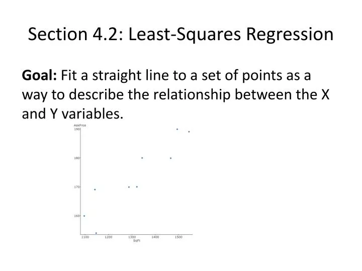
Section 4.2: Least-Squares Regression Goal: Fit a straight line to a set of points as a way to describe the relationship between the X and Y variables.
Asking price in thousands of dollars Dec.2010 data, Naples, FL. (Problem 28 in text)
y = mx + b → AskPrice = 0.0686 × SqFt + 83.2366 y = → AskPrice = 83.2366 + 0.0686 × SqFt
Residual = Observed – Predicted Least-squares line minimizes “sum of the squared residuals”
y = mx + b → AskPrice = 0.0686 × SqFt + 83.2366 y = → AskPrice = 83.2366 + 0.0686 × SqFt SLOPE For each one square foot increase, we expect the average asking price to be 0.0686 higher. (0.0686 = $68.60) INTERCEPT A zero square foot home would have an asking price of 83 .2366 (83 .2366 =$83,236.60) This example of the intercept is extrapolation. It is a bad idea to extrapolate outside of your range of data. Interpretation
y = mx + b → AskPrice = 0.0686 × SqFt + 83.2366 y = → AskPrice = 83.2366 + 0.0686 × SqFt Suppose X=1344 square feet, Y= 180.0 83.2366 + 0.0686 × 1344 = 175.435 Predicted Y= Predicted Cost= $175,435 Residual = observed – predicted = 180.0 – 175.435 = 4.565 How to calculate predicted value and residuals
For a good applet to explore leverage and correlation see: http://www.calpoly.edu/~srein/StatDemo/All.html