Download
1 / 49
500 likes | 644 Views
Introduction to Parallel Computing. Parallel Computing. Traditionally, software is written for a uniprocessor machine Executed by a single computer with one CPU Instructions are executed sequentially, one after the other

E N D
Parallel Computing • Traditionally, software is written for a uniprocessor machine • Executed by a single computer with one CPU • Instructions are executed sequentially, one after the other • In CS221 we briefly touched upon how this is not quite true; there is pipelining and today’s uniprocessors generally have multiple execution units and try to run many instructions in parallel • Parallel computing is the simultaneous use of multiple resources to run a program
Where are the computing resources? • The compute resources can include: • A single computer with multiple execution units • A single computer with multiple processors • A network of computers • A combination of the above • Our Beowulf cluster, beancounter.math.uaa.alaska.edu, is in this category
Applying Parallel Programming • To be effectively applied, the problem should generally have the following properties: • Broken apart into discrete pieces of work that can be solved simultaneously • Execute multiple program instructions at any moment in time • Solved in less time with multiple compute resources than with a single compute resource • Is a problem that runs too long on a uniprocessor or is too large for a uniprocessor (e.g. memory constraints)
Typical Parallel Programming Problems • Motivated by scientific problems, numerical simulation, “supercomputer” problems: • weather and climate • chemical and nuclear reactions • biological, human genome • geological, seismic activity http://aeff.uaa.alaska.edu
MIMD • Multiple Instruction: every processor may be executing a different instruction stream • Multiple Data: every processor may be working with a different data stream • Execution can be synchronous or asynchronous • Examples: most current supercomputers, networked parallel computer "grids" and “clusters” and multi-processor SMP computers
Some Parallel Computer Architectures • Shared Memory • Multiple processors share the same global memory • Change made to memory by one CPU visible by all others
Shared Memory Architecture • Uniform Memory Access (UMA) • Most commonly represented today by Symmetric Multiprocessor (SMP) machines • Identical processors • Equal access and access times to memory • Sometimes called CC-UMA - Cache Coherent UMA. Cache coherent means if one processor updates a location in shared memory, all the other processors know about the update. Cache coherency is accomplished at the hardware level.
Shared Memory Architecture • Non-Uniform Memory Access (NUMA) • Often made by physically linking two or more SMPs • One SMP can directly access memory of another SMP • Not all processors have equal access time to all memories • Memory access across link is slower • If cache coherency is maintained, then may also be called CC-NUMA - Cache Coherent NUMA
Shared Memory Architecture • Advantages • Global address space provides a user-friendly programming perspective to memory • Data sharing between tasks is both fast and uniform due to the proximity of memory to CPUs • Disadvantages • Lack of scalability between memory and CPUs. Adding more CPUs can geometrically increases traffic on the shared memory-CPU path, and for cache coherent systems, geometrically increase traffic associated with cache/memory management. • Programmer responsibility for synchronization constructs that insure "correct" access of global memory. • Expense: it becomes increasingly difficult and expensive to design and produce shared memory machines with ever increasing numbers of processors.
Some Parallel Computer Architectures • Distributed Memory • Processors have their own local memory. Memory addresses in one processor do not map to another processor, so there is no concept of global address space across all processors. • Because each processor has its own local memory, it operates independently. Changes it makes to its local memory have no effect on the memory of other processors. Hence, the concept of cache coherency does not apply.
Distributed Memory • When a processor needs access to data in another processor, it is usually the task of the programmer to explicitly define how and when data is communicated. Synchronization between tasks is likewise the programmer's responsibility. • The network "fabric" used for data transfer varies widely, though it can can be as simple as Ethernet.
Distributed Memory • Advantages: • Memory is scalable with number of processors. Increase the number of processors and the size of memory increases proportionately. • Each processor can rapidly access its own memory without interference and without the overhead incurred with trying to maintain cache coherency. • Cost effectiveness: can use commodity, off-the-shelf processors and networking. • Disadvantages: • The programmer is responsible for many of the details associated with data communication between processors. • It may be difficult to map existing data structures, based on global memory, to this memory organization. • Non-uniform memory access (NUMA) times
Combination • The largest and fastest machines today use a combination of shared and distributed architectures
Parallel Programming Models • Data Parallel • Like SIMD approach • Shared Memory • Threads • Message Passing
Shared Memory Programming • In the shared-memory programming model, tasks share a common address space, which they read and write asynchronously. • Various mechanisms such as locks and semaphores may be used to control access to the shared memory. • An advantage of this model from the programmer's point of view is that the notion of data "ownership" is lacking, so there is no need to specify explicitly the communication of data between tasks. Program development can often be simplified. • An important disadvantage in terms of performance is that it becomes more difficult to understand and manage data locality. • No common implementation of shared memory programming exists today beyond a handful of CPU’s
Thread Model • A single process can have multiple, concurrent execution paths • A thread's work may best be described as a subroutine within the main program. Any thread can execute any subroutine at the same time as other threads. • Threads communicate with each other through global memory (updating address locations). • Requires synchronization constructs to insure that more than one thread is not updating the same global address at any time. Studied in OS class
Message Passing • Characteristics: • A set of tasks that use their own local memory during computation. Multiple tasks can reside on the same physical machine as well across an arbitrary number of machines. • Tasks exchange data through communications by sending and receiving messages. • Data transfer usually requires cooperative operations to be performed by each process. For example, a send operation must have a matching receive operation.
Message Passing Programming • From a programming perspective, message passing implementations commonly comprise a library of subroutines that are imbedded in source code. The programmer is responsible for determining all parallelism. • History: • A variety of message passing libraries have been available since the 1980s, but no standard • In 1992, the MPI Forum was formed with the primary goal of establishing a standard interface for message passing implementations. • Part 1 of the Message Passing Interface (MPI) was released in 1994. Part 2 (MPI-2) was released in 1996. • MPI is now the "de facto" industry standard for message passing, replacing virtually all other message passing implementations used for production work. MPI-2 full implementation rare.
Constructing Parallel Code • Hard to do • Fully Automatic Approach – parallelizing compiler • The compiler analyzes the source code and identifies opportunities for parallelism. • The analysis includes identifying inhibitors to parallelism and possibly a cost weighting on whether or not the parallelism would actually improve performance. • Loops (do, for) loops are the most frequent target for automatic parallelization. • Programmer Directed • Using "compiler directives" or possibly compiler flags, the programmer explicitly tells the compiler how to parallelize the code. • Generally much better performance than automatic • May be able to be used in conjunction with some degree of automatic parallelization also.
Designing Parallel Programs • First step: Understand the problem • If you are starting with a serial program, this necessitates understanding the existing code also. • Before spending time in an attempt to develop a parallel solution for a problem, determine whether or not the problem is one that can actually be parallelized. • Example of Parallelizable Problem: Calculate the potential energy for each of several thousand independent conformations of a molecule. When done, find the minimum energy conformation. • Example of a Non-parallelizable Problem: Calculation of the Fibonacci series (1,1,2,3,5,8,13,21,...) by use of the formula: F(k + 2) = F(k + 1) + F(k)
Understanding the Problem • Identify the program's hotspots: • Know where most of the real work is being done. The majority of scientific and technical programs usually accomplish most of their work in a few places. • Profilers and performance analysis tools can help here • Focus on parallelizing the hotspots and ignore those sections of the program that account for little CPU usage. • Identify bottlenecks in the program • Are there areas that are disproportionately slow, or cause parallelizable work to halt or be deferred? • May be possible to restructure the program or use a different algorithm to reduce or eliminate unnecessary slow areas • Identify inhibitors to parallelism. One common class of inhibitor is data dependence, as demonstrated by the Fibonacci sequence above. • Investigate other algorithms if possible. This may be the single most important consideration when designing a parallel application.
Designing Parallel Programs • One of the first steps in designing a parallel program is to break the problem into discrete "chunks" of work that can be distributed to multiple tasks. This is known as decomposition or partitioning. • There are two basic ways to partition computational work among parallel tasks: domain decomposition and functional decomposition
Domain Decomposition • the data associated with a problem is decomposed. Each parallel task then works on a portion of the data.
Domain Decomposition • Sample ways to split up arrays
Functional Decomposition • The focus is on the computation that is to be performed rather than on the data manipulated by the computation. The problem is decomposed according to the work that must be done. Each task then performs a portion of the overall work. e.g. climate model: The atmosphere model generates wind velocity data that are used by the ocean model, the ocean model generates sea surface temperature data that are used by the atmosphere model, etc.
Hybrid Decomposition • In many cases it may be possible to combine the functional and domain decomposition approaches. • E.g. weather model • Spatial area to process • Functions to process
Communications • The need for communications between tasks depends upon your problem: • You DON'T need communications • Some types of problems can be decomposed and executed in parallel with virtually no need for tasks to share data. • E.g. inverting an image • These types of problems are often called embarrassingly parallel because they are so straight-forward. Very little inter-task communication is required. • You DO need communications • Most parallel applications are not quite so simple, and do require tasks to share data with each other. • E.g. a 3-D heat diffusion problem requires a task to know the temperatures calculated by the tasks that have neighboring data. Changes to neighboring data has a direct effect on that task's data.
Important Communications Factors • Cost of communications • Inter-task communication virtually always implies overhead. • Machine cycles and resources that could be used for computation are instead used to package and transmit data. • Communications frequently require some type of synchronization between tasks, which can result in tasks spending time "waiting" instead of doing work. • Competing communication traffic can saturate the available network bandwidth, further aggravating performance problems.
Important Communications Factors • Consider latency and bandwidth of your network • Sending many small messages can cause latency to dominate communication overheads. Often it is more efficient to package small messages into a larger message, thus increasing the effective communications bandwidth. • Synchronous vs. asynchronous communications • Requires some type of "handshaking" between tasks that are sharing data. This can be explicitly structured in code by the programmer, or it may happen at a lower level unknown to the programmer. • Often referred to as blocking communications • Asynchronous communications allow tasks to transfer data independently from one another. For example, task 1 can prepare and send a message to task 2, and then immediately begin doing other work. When task 2 actually receives the data doesn't matter. • Asynchronous communications are often referred to as non-blocking communications. Interleaving computation with communication is the single greatest benefit for using asynchronous communications.
Scope of Communications • Knowing which tasks must communicate with each other is critical during the design stage of a parallel code. • Point-to-point - involves two tasks with one task acting as the sender/producer of data, and the other acting as the receiver/consumer. • Collective - involves data sharing between more than two tasks, which are often specified as being members in a common group, or collective. Some common variations:
Synchronization • Barrier • Usually implies that all tasks are involved • Each task performs its work until it reaches the barrier. It then stops, or "blocks". • When the last task reaches the barrier, all tasks are synchronized. • What happens from here varies. Often, a serial section of work must be done. In other cases, the tasks are automatically released to continue their work. • Lock / semaphore • Can involve any number of tasks • Typically used to serialize (protect) access to global data or a section of code. Only one task at a time may use (own) the lock / semaphore / flag. • Other tasks can attempt to acquire the lock but must wait until the task that owns the lock releases it. • Synchronous communication operations • Involves only those tasks executing a communication operation • E.g. only send after ack received
Load Balancing • Load balancing refers to the practice of distributing work among tasks so that all tasks are kept busy all of the time. It can be considered a minimization of task idle time. • Load balancing is important to parallel programs for performance reasons.
Achieving Load Balance • Equally partition the work each task receives • Data, loop iterations similar for each CPU • Use dynamic work assignment • Certain classes of problems result in load imbalances even if data is evenly distributed among tasks: • Sparse arrays - some tasks will have actual data to work on while others have mostly "zeros". • N-body simulations – where most of the particles are in one place • May be helpful to use a scheduler - task pool approach. As each task finishes its work, it queues to get a new piece of work. • It may become necessary to design an algorithm that detects and handles load imbalances as they occur dynamically within the code.
Granularity of Parallelism • Ratio of computation to communication • Fine-grained • Small amounts of computational work are done between communication events • Low computation to communication ratio • Facilitates load balancing • Bad on communication overhead • Coarse-grained • Relatively large amounts of computational work are done between communication/synchronization events • High computation to communication ratio • Implies more opportunity for performance increase • Harder to load balance efficiently
Parallel Array Example • Independent calculations on 2D array Serial code: for i = 1 to n for j = 1 to m a[i,j] = fcn(a[i,j])
One Solution • Master process • Initializes array • Splits array into rows for each worker process • Sends info to worker processes • Wait for results from each worker • Worker process receives info, performs its share of computation and sends results to master. • Master displays the results
Solution Pseudocode Find out if I am MASTER or WORKER if I am MASTER { initialize the array send each WORKER info on part of array it owns send each WORKER its portion of initial array receive from each WORKER results } else if I am WORKER { receive from MASTER info on part of array I own receive from MASTER my portion of initial array for i = myfirstrow to mylastrow for j = 1 to m a[i,j] = fcn(a[i,j]) send MASTER results , i.e. a[myfirstrow,*] to a[mylastrow,*] }
Parallel Example • 1D wave on a string • The amplitude on the y axis • i as the position index along the x axis • node points imposed along the string • update of the amplitude at discrete time steps.
Wave Solution • The entire amplitude array is partitioned and distributed as subarrays to all tasks. Each task owns a portion of the total array. • Load balancing: all points require equal work, so the points should be divided equally • A block decomposition would have the work partitioned into the number of tasks as chunks, allowing each task to own mostly contiguous data points. • Communication need only occur on data borders. The larger the block size the less the communication. “ghost” data
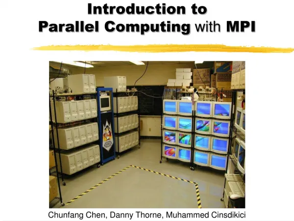
MPI • Common implementation • Cluster of machines connected by some network • Could be the Internet, but generally some type of high-speed LAN • Share same file system • One machine designated as the Master, others are slaves or workers
MPI • Program skeleton: #include<mpi.h> void main(int argc, char *argv[]) { int rank,size; MPI_Init(&argc, &argv); MPI_Comm_rank(MPI_COMM_WORLD,&rank); MPI_Comm_size(MPI_COMM_WORLD,&size); /* ... your code here ...*/ MPI_Finalize(); } Like an array, separate instance on each processor Get process ID starting at 0 Get number of processes
MPI Hello, World #include <stdio.h> #include "mpi.h" main(int argc, char **argv) { int my_rank; int p; int source; int dest; int tag=50; char message[100]; MPI_Status status; MPI_Init(&argc,&argv); MPI_Comm_rank(MPI_COMM_WORLD, &my_rank); MPI_Comm_size(MPI_COMM_WORLD, &p);
MPI Hello, World if (my_rank == 1) { printf("I'm number 1!\n"); sprintf(message,"Hello from %d!", my_rank); dest=0; MPI_Send(message,strlen(message)+1, MPI_CHAR, dest, tag, MPI_COMM_WORLD); } else if (my_rank !=0) { sprintf(message,"Greetings from %d!", my_rank); dest=0; MPI_Send(message,strlen(message)+1, MPI_CHAR, dest, tag, MPI_COMM_WORLD); } else { for (source =1; source <p; source++) { MPI_Recv(message, 100, MPI_CHAR, source, tag, MPI_COMM_WORLD,&status); printf("%s\n",message); } } MPI_Finalize(); return 0; }
MPI Reduce Example #include <stdio.h> #include <mpi.h> int main (int argc, char *argv[]) { int rank, value, recv, min, root; MPI_Init(&argc, &argv); MPI_Comm_rank(MPI_COMM_WORLD,&rank); value=rank+1; root=0; MPI_Reduce(&value,&recv,1,MPI_INT,MPI_SUM,root,MPI_COMM_WORLD); if (rank==root) printf("Sum=%d\n",recv); MPI_Barrier(MPI_COMM_WORLD); MPI_Reduce(&value,&min,1,MPI_INT,MPI_MIN,root,MPI_COMM_WORLD); if (rank==root) printf("Min=%d\n",min); MPI_Finalize(); return 0; }
Beancounter examples • Heatbugs • Genetic Algorithm
References • http://www.llnl.gov/computing/tutorials/parallel_comp/ • http://www.osc.edu/hpc/training/mpi/raw/fsld.002.html • http://www.math.uaa.alaska.edu/~afkjm/cluster/beancounter/