Download
1 / 51
510 likes | 924 Views
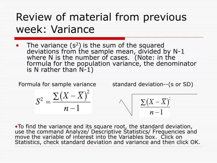
Review of material from previous week: Variance. The variance (s 2 ) is the sum of the squared deviations from the sample mean, divided by N-1 where N is the number of cases. (Note: in the formula for the population variance, the denominator is N rather than N-1). Formula for sample variance.

E N D
Review of material from previous week: Variance • The variance (s2)is the sum of the squared deviations from the sample mean, divided by N-1 where N is the number of cases. (Note: in the formula for the population variance, the denominator is N rather than N-1) Formula for sample variance standard deviation--(s or SD) • To find the variance and its square root, the standard deviation, use the command Analyze/ Descriptive Statistics/ Frequencies and move the variable of interest into the Variables box. Click on Statistics, check standard deviation and variance and then click OK.
Review from previous week: Standard deviation and normal distribution • The standard deviation is the square root of the variance. It measures how much a typical case departs from the mean of the distribution. The size of the SD is generally about one-sixth the size of the value of the range • The standard deviation becomes meaningful in the context of the normal distribution. In a normal distribution • The mean, median and mode of responses for a variable coincide • The distribution is symmetrical in that it divides into two equal halves at the mean, so that 50% of the scores fall below the mean and 50% above it (sum of probabilities of all categories of outcomes = 1.0 (total “area” = 1) • 68.26 % of the scores in a normal distribution fall within plus or minus one standard deviation of the mean.95.44% fall within 2 SDs. The curve has a standard deviation of 1 • Thus we are able to use the SD to assess the relative standing of a score within a distribution, to say that it is 2 SDs above or below the average, for example • The normal distribution has a skewness equal to zero • Some normal curves in nature: heights within gender; LDL cholesterol
Review from last week: Histogram with superimposed normal curve • Histogram of the “vehicle weight” variable with a superimposed curve. This is what a normal distribution of a variable with the same mean and standard deviation would look like. This distribution has a positive skew and is more platykurtic • Definition: “Kurtosis is a measure of whether the data are peaked or flat relative to a normal distribution. That is, data sets with high kurtosis tend to have a distinct peak near the mean, decline rather rapidly, and have heavy tails. Data sets with low kurtosis tend to have a flat top near the mean rather than a sharp peak. A uniform distribution would be the extreme case.”
Descriptive vs. Inferential Statistics • Descriptive statistics: such measures as the mean, standard deviation, correlation coefficient when used to summarize sample data and reduce it to manageable proportions • Inferential (sampling) statistics: use of sample characteristics to infer parameters or properties of a population on the basis of known sample results. Based on probability theory. Statistical inference is the process of estimating parameters from statistics. • Inferential statistics require that certain assumptions be met about the nature of the population.
Assumptions of Inferential Statistics • Let’s consider an example of an application of parametric statistics, the t-test. Suppose we have drawn a sample of Chinese Americans and a sample of Korean Americans and have a belief that the two populations are likely to differ in their attitudes toward aging. The purpose of the t-test is to determine if the means of the populations from which these two samples were drawn are significantly different. There are certain assumptions that have to be met before you can perform this test: • You must have at least interval level data • The data from both samples have to represent scores on the same variable, that is, you can’t measure attitudes toward aging in different ways in different populations • The populations from which the samples are drawn are normally distributed with respect to the variable • The variances of the two populations are equal • The samples have been randomly drawn from comprehensive sampling frames; that is, each element or unit in the population has an equal chance of being selected (random sampling permits us to invoke statistical theories about the relationships of sample and population characteristics)
Population Parameters vs. Sample Statistics • Purpose of statistical generalizations is to infer the parameters of a population from statistics known about a sample drawn from the population • Greek letters usually refer to population characteristics: population standard deviation = σ, • population mean = µ • Roman letters usually refer to sample characteristics: sample standard deviation = s, sample mean = The formula for the variance in a population is: The formula for the variance in a sample is:
Frequency Distributions vs. Probability Distributions Tails, heads or Heads, tails • The general way in which statistical hypothesis testing is done is to compare obtained frequencies to theoretical probabilities. • Compare the probability distribution for number of heads in two, four and 12 coin flips vs. an actual example of coin flipping. (from D. Lane, “History of Normal Distribution” Heads, heads Tails, tails Formula for binomial probabilities
Comparing Obtained to Theoretical Outcomes • If you did a sample experiment and you got, say, two heads in two flips 90% of the time you would say that there was a very strong difference between the obtained frequencies and the expected frequencies, or between the obtained frequency distribution and the probability distribution • Over time, if we were to carry out lots and lots of coin-flipping experiments, the occasions when we got 90% occurrence of two heads in two flips would start to be balanced out by results in the opposite direction, and eventually with enough cases our obtained frequency distribution would start to look like the theoretical probability distribution. For an infinite number of experiments, the frequency and probability distributions would be identical.
Significance of Sample Size • Central Limit Theorem: the larger the sample size, the greater the probability that the obtained sample mean will approximate the population mean • Another way to put it is that the larger the sample size, the greater the likelihood that the sample distribution will approximate the shape of a normal distribution for a variable with that mean and standard deviation
Reasoning about Populations from Sample Statistics • Parameters are fixed values and are generally unknown • Statistics vary from one sample to another, are known or can be computed • In testing hypotheses, we make assumptions about parameters and then ask how likely our sample statistics would be if the assumptions we made were true • It’s useful to think of an hypothesis as a prediction about an event that will occur in the future, that we state in such a way that we can reject that prediction • We might reason that if what we assume about the population and our sampling procedures are correct, then our sample results will usually fall within some specified range of outcomes.
Reasoning about Populations from Sample Statistics • If our sample results fall outside this range into a critical region, we must reject our assumptions. • For example, if we assume that two populations, say males and females, have the same views on increasing the state sales tax but we obtain results from our randomly drawn samples indicating that their mean scores on the attiitude toward sales tax measure are so different that this difference falls into the far reaches of a distribution of such sample differences, we would have to reject our assumption that the populations do not differ. But our decision would have a lot to do with how we defined the “far reaches” of this distribution, called the “critical region.”
Reasoning about Populations from Sample Statistics, cont’d • We can say that we have carried out statistical hypothesis testing if • We have allowed for all potential outcomes of our experiment or survey results ahead of the test • We have committed beforehand to a set of procedures or requirements that we will use to determine if the hypothesis should be rejected and • We agree in advance on which outcomes would mean that the hypothesis should be rejected • Probability theory lets us assess the risk of error and take these risks into account in making a determination about whether the hypothesis should be rejected
Types of Error • Error risks are of two types: • Type I error, also called alpha (α) error, is the risk of rejecting the null hypothesis (H0:hypothesis of no difference between two populations, or no difference between the sample mean and the population mean) when it is in fact true. (we set our confidence level too low) • Type II error, or beta (β) error, is the risk of failing to reject a null hypothesis when it is in fact false. (set our confidence level too high) • When we report the results of our test, it is often expressed in terms of the degree of confidence we have in our result (for example, we are confident that there is less than a 5% or 2.5% or 1% probability that the result we got was obtained by chance and that in fact we should fail to reject the null hypothesis. This is usually referred to as the confidence level or the significance level.
Why We are Willing to Generalize from Sample Data • Why should we generalize on the basis of limited information? • Time and cost factors • Inability to define a population and list all of its elements • Random sampling: every member of the population has an equal chance of being selected for the sample • Theoretically, to do this requires that you have a list of all the members of the population • To survey the full-time faculty at UPC, for example, you might obtain a list of all the faculty, number them from one to N, and then use a random number table to draw the numbered cases for your sample. • Random sampling can be done with and without replacement • SPSS will draw a random sample for you from your list of cases (Data/Select Cases/Random Sample of Cases) of a desired size
Normal Distribution, a Review • The normal curve is an essential component of decision-making by which you can generalize your sample results to population parameters • Notion of the “area under the normal curve” the area between the curve and the baseline which contains 100% of the cases
Characteristics of the normal curve, cont’d • Constant proportion of the area under the curve will lie between the mean and a given point on the baseline expressed in standard score units (Zs), and this holds in both directions (both above and below the mean). That is, for any given distance in standard (sigma) scores the area under the curve (proportion of cases) will be the same both above and below the mean • The most commonly occurring scores cluster around the mean, where the curve is the highest, while the extremely high or extremely low scores occur in the tails and become increasingly rare (the height of the curve is lower and in the limit approaches the baseline. The total area (sum of individual probabilities) sums to 1.0
Table of the Area under the Normal Curve • Tables of the Area under the Normal Curve are available in your supplemental readings, p. 469 in Kendrick and p. 299 in Levin and Fox, and can be found on the Web. • You can use this table to find out the area under the normal curve (the proportion of cases) which theoretically are likely to fall between the population mean and some score expressed in standard unit or Z scoress. • For example, let’s find what proportion of cases in a normal distribution would lie between the population mean and a standard score of 2.2 (that is, a score on the variable that is 2.2 standard deviations above the mean-also called a Z score)
Z Scores and the Normal Table • In the normal table you look up the Z score of 2.2 and to the right of that you will find the proportional “area between the mean and Z”, which is .4861. Thus 48.61% of the cases in the normal distribution lie between the mean and Z=2.2. • What proportion of cases lie below this? Add 50% to 48.61% (because 50% of the cases lie below the mean). • What proportion of cases lie above this? 100% (100% of cases) minus 50% + 48.61%, or 1.39% of cases • What proportion of cases lie between -2.2 and +2.2? • Some Tables will express the values in percentages, some in proportions.
Using the Mean and Standard Deviation to find Where a Particular Value Might Fall • Let’s consider the “vehicle weight” variable from the cars. sav file. From a previous analysis we learned that the distribution looked like this histogram on the right and it had the sample statistics reported in the table, including a mean of 2969.56 and a standard deviation of 849.827. What would be the weight of a vehicle that was one standard deviation above the mean? Add one sd to the mean, and you get 3819.387 One standard deviation below the mean?subtract one sd from the mean, and you get 2119.733 • What percent of vehicles have weights between those two values, assuming a random, representative sample and no measurement error? 68.26 • What would be the weight of a vehicle that was two standard deviations above the mean? Two standard deviations below the mean? What percent of vehicles have weights between those two values, assuming a random, representative sample and no measurement error? 95.44%
Z Scores • The Z score expresses the relationship between the mean score on the variable and the score in question in terms of standardized units (units of the standard deviation) • Thus from the calculations we just did we can say that the value of vehicle weight of 3819.387 has a Z score of +1 and the weight of 2119.733 has a Z score of -1 • Turning the question around, suppose we wanted to know where in the distribution we would find a car that weighed 4500 pounds. To answer that question we would need to find the Z score for that value. The computing formula for finding a Z score is Thus, the z score for the vehicle weight 4500 pounds (X) is 4500-2969.56 (the mean)/849.827 (the standard deviation), or Z=1.80. What about a 1000-lb car? (Z=-2.31)
How to Interpret and Use the Z Score: Table of the Area under the Normal Curve • Suppose we know that a vehicle weight has a Z score of +1 (is 1SD above the mean). Where does that score stand in relation to the other scores? • Let’s think of the distribution image again. Recall that we said that half of the cases fall below the mean, and that 34.13% of the cases fall between the mean and one SD below it, and 34.13% of the cases fall between the mean and one sd above it. So if a vehicle weight has a Z score of +1, what proportion of cases are above and what percent are below it? Let’s look at the next slide
Table of the Area under the Normal Curve, continued Consider the z score of 1.00. .3413 of scores lie between z and the mean; .1587 of scores lie above a z of 1.00, and .8413 lie below it. Now suppose z was -1.0. .3413 of scores would still lie between z and the mean; what percent of scores would lie above it and below it? Remember that the normal distribution is symmetrical
Sampling Distribution of Sample Means and the Standard Error of the Mean • The characteristics of populations, or parameters, are usually not known. All we can do is estimate them from sample statistics. What gives us confidence that a sample of, say, 100 or 1000 people permits us to generalize to millions of people? • The key concept is the notion that theoretically we could draw all possible samples from the population of interest and that for the sample statistics that we collect, such as the mean, there will be a sampling distribution with its own mean and standard deviation. In the case of the mean, this is called the sampling distribution of sample means, and its mean is represented as µ • Characteristics: (1) approximates a normal curve (2) its mean is equal to the population mean (3) its standard deviation is smaller that that of the population (sample mean more stable than scores which comprise it) • We can also estimate the standard deviation of the sampling distribution of sample means, which would give us an indicator of the amount of variability in the distribution of sample means. This value, known as the standard error of the mean, is represented by the symbol σBasically, it tells you how much statistics can be expected to deviate from parameters when sampling randomly from the population
Estimating the Standard Error • The standard error of the mean is hypothetical and unknowable; consequently we estimate it with sample statistics using the formula: standard deviation of the sample divided by the square root of the sample size. (SPSS uses N in the denominator; Levin and Fox advocate N-1 for obtaining an unbiased estimate of the standard error Makes little difference with large N) As you will quickly note, the standard error is very sensitive to sample size, such that the larger the sample size, the smaller the error. And the smaller the error, the greater the homogeneity in the sampling distribution of sample means (that is, if the standard error is small relative to the range, the sample means aren’t all over the place). The standard error is of importance primarily because it is used in the calculation of other inferential statistics and when it is small it increases the confidence you can have that your sample statistics are representative of population parameters.
Finding Z Scores and the Standard Error with SPSS • Let’s calculate Z scores and standard errors for the variables companx1 and companx3 in the Lesson3.sav data set • Go to Anayze/Descriptive Statistics/ Descriptives • Move the variables companx3 (difficulty understanding the technical aspects of computers) and companx1(fear of making mistakes) into the Variables window using the black arrow • Click on “Save standardized values as variables” (this creates two new variables whose data are expressed in Z scores rather than raw scores) • Click options and check “S. E. Mean” as well as mean, s, etc • Click Continue and then OK • Go to the Output viewer to see descriptive statistics for the variables • Go to the Data Editor and note the new variables which have been added in the right-most columns
Compare S.E.s, Raw Scores to Z Scores Note that the standard errors of the two variables are about the same although the range is larger for “difficulty understanding” Raw scores Z scores.
Point Estimates, Confidence Intervals • A point estimate is an obtained sample value such as a mean, which can be expressed in terms of ratings, percentages, etc. For example, the polls that are released showing a race between two political candidates are based on point estimates of the percentage of people in the population who intend to vote for or at least favor one or the other candidate • Confidence level and confidence interval • A confidence interval is a range that the researcher constructs around the point estimate of its corresponding population parameter, often expressed in the popular literature as a “margin of error” of plus or minus some number of points, percentages, etc. This range becomes narrower as the standard error becomes smaller, which in turn becomes smaller as the sample size becomes larger
Confidence levels • Confidence levels are usually expressed in terms like .05, .01, etc. in the scholarly literature, and 5%, 1% etc in the popular press. They are also called significance levels. They represent the likelihood that the population parameter which corresponds to the point estimate falls outside that range. To turn it around the other way, the represent the probability that if you constructed 100 confidence intervals around the point estimate from samples of the same size, 95 (or 99) of them would contain the true percentage of people in the population who preferred Candidate A (or Candidate B)
Using the Sample Standard Error to Construct a Confidence Interval • Since the mean of the sampling distribution of sample means for a particular variable equals the population mean for that variable, we can try to estimate how likely it is that the population mean falls within a certain range, using the sample statistics. • We will use the standard error of the mean from our sample to construct a confidence interval around our sample mean such that there is a 95% likelihood that the range we construct contains the population mean
Calculating the Standard Error with SPSS • Let’s consider the variable “vehicle weight” from the Cars.sav data file. • Let’s find the mean and the standard error of the mean for “vehicle weight” • Go to Analyze/Descriptive Statistics/ Frequencies, then click the Statistics button and request the mean and the standard error of the mean (S. E. Mean)
Constructing the Confidence Interval Upper and Lower Limits • Now let’s construct a confidence interval around the mean of 2969.56 such that we can have 95% confidence that the population mean for the variable “vehicle weight” will fall within this range. • We are going to do this using our sample statistics and the table of Z scores (area under the normal curve). To obtain the upper limit of the confidence interval, we take the mean (2969.56) and add to it (Z X S.E)) where Z is the z-score corresponding to the area under the normal curve representing the amount of risk we’re willing to take (for example 5%, or, we want to be 95% confident that the population mean falls within the confidence interval) and S.E. is our sample standard error (42.176)
Formulas for computing confidence intervals around an obtained sample mean • Formulas for Upper and Lower Limits of the Confidence Interval • Upper Limit: Sample Mean plus (Z times the standard error), where Z corresponds to the desired level of confidence • Lower Limit: Sample Mean minus (Z times the standard error), where Z corresponds to the desired level of confidence
Consult the Table of the Area under the Normal Curve • In the normal table look until you find the figure .025. You will note that this is one-half of 5%. Since we have to allow for the possibility that the population mean might fall in either of the two tails of the distribution we have to cut our risk area under the normal curve in half, hence .025. An area under the curve such that only .025 percent of cases, in either tail of the distribution, would fall that far from the mean, corresponds to a Z of 1.96
Another normal table; Z corresponding to 95% confidence interval (two tailed) = 1.96 (this table shows area beyond Z)
Calculations for the Confidence Interval • Now, compute the upper limit of the confidence interval (this represents the largest value (CIu)that you are able to say, with 95% confidence, that the population mean vehicle weight could take. 2969.56 + (1.96 (the Z score)(42.176 the standard error) = 3052 • Now, compute the lower limit of the confidence interval (this represents the lowest value that you are able to say, with 95% confidence, that the population mean vehicle weight could take (CIl). 2969.56 – (1.96) (42.176) = 2886 • Thus we can say with 95% confidence that the mean vehicle weight in the population falls within the range 2886-3052
Constructing the Confidence Interval in SPSS • Now run this analysis using SPSS • Go to Analyze/ Descriptive Statistics/ Explore. Put Vehicle Weight into the Dependent List box. Click on Statistics and choose Descriptives and set the confidence interval for the mean at 95%. Click Continue and then OK. • Compare your output Lower Bound and Upper Bound to the figures you did by hand. Because you may not have gotten all the significant digits for the mean and standard error your figures may be off a tiny bit
Examining your SPSS Output Here’s what your output should look like: Now rerun the analysis to find the confidence interval for the 99% level of confidence. But before you do, consult the table of the area under the normal curve and see if you can figure out what the value of Z should be by which you would multiply the S.E. of the mean (hint: divide .01 by 2, for each of the two tails of the distribution)
Finding the 99% confidence interval Interpolate in the table to find the z score corresponding to the 99% confidence interval (that is, there’s only a 1% probability (.005 in each tail of the distribution) that the population parameter falls outside the stated range
Output for 99% Confidence Level Your output for the 99% confidence level should like this Were you able to figure out the correct value of Z from the normal table? You have to interpolate between .0051 and .0049. Z equals approximately 2.58. That is, at a Z score of + or – 2.575, only about .005 of the means will fall above (or below) that score in the sampling distribution Write a sentence reporting your findings, indicating how confident you are (and what you are confident about), e.g., we can state with XXX confidence that mean population vehicle weight is between XXX and XXX
Some Commonly Used Z Values • A quick chart of Z values for “two-tailed” tests • 95% confidence level: Z = 1.96 • 99% confidence level: Z = 2.575 • 99.9 confidence level: Z = 3.27 • Note that these values are appropriate when we want to put upper and lower limits around our point estimate. On other occasions we will not be interested in both “tails” of the distribution but only in, say, the upper tail (the upper 5% of the distribution) and so the Z score would be different. Look up in the table to see what the z score corresponding to the upper 5 percent of the sampling distribution would be. For example, if we assume that the population mean is zero and we get a sample value so much higher that the corresponding Z score is in the upper 5 percent, we might conclude that the sample score did not come from the population whose mean is zero.
Confidence Intervals and Levels for Percentage and Proportion Data • Using a sample percentage as a point estimate we can construct a confidence interval around the estimate such that we can say with 95% confidence that the corresponding population parameter falls within a certain range • The first thing we need is an estimate of the standard error of proportions, similar in concept to the standard error of sample means in that there is a sampling distribution of sample proportions which will be normal • The standard error of proportions is the standard deviation of the sampling distribution of sample proportions
Computing Formula for Standard Error of Proportions from Sample Data • The formula for computing the population standard error of proportions, σp , from the sample data is σp where p is the proportion of cases endorsing option A, for example, those preferring candidate A rather than B. (1-p) is also seen as q in some formulas. Thus the standard error of proportions in a sample with 10 cases where .60 of the respondents preferred Candidate A and .40 preferred Candidate B is the square root of (.60)(.40)/10 or .1549 (Note: example on p. 258 in Kendrick has typo in it. Denominator P (1-P) should equal .2281, not .2881. The correct standard error of proportions for the example in the text is .0124) σp
Putting Confidence Intervals Around a Sample Proportion • Continuing with our example, we want to find the upper and lower bounds for a confidence interval around the sample proportion p of .60 in favor of Candidate A. What can we say with 95% confidence is the interval within which the corresponding parameter in the population will fall? • CIupper = P + (Z)( σ) or .60 +(1.96 X .1549) or .904 • CIlower = P - (Z)( σ) or .60 – (1.96 X .1549) or .296 • Thus the proportion in the population which favors Candidate A could range anywhere from .296 to .904, and we are 95% confident in saying that!!! What do you think our problem is? How could we narrow the range?
Using Dummy Variables to Find Confidence Intervals for Proportion • A dummy variable is one on which each case is coded for either presence or absence of the attribute. For example, we could recode the ethnicity data into the dummy variable “whiteness” or “Chinese-ness” so that every case would have either a 1 or a zero on the variable. All of the white (or Chinese) respondents would get a 1 and the others would get a zero on the variable. • Let’s create a dummy variable for the variable “Country of origin” in the Cars.sav data set. The new dummy variable will be “American in Origin.” If you look at the country of origin variable in the Variable View you will see that it is coded as 1 = American, 2 = European, and 3 = Japanese. We are going to recode it into a new dummy variable where all of the American cars get a “1” and the Japanese and European cars all get a zero.
Creating a Dummy Variable • In SPSS go to Transform/Recode/Into Different Variables • Move the “Country of Origin” variable into the Numeric Variable window. In the Ouput Window give the new variable the name “AmerOrig” and the label “RecodedCountryofOriginVariable.” click Change • Click on the “Old and New Values” button and recode the old variable such that a value of 1 from the old equals 1 in the new, and values in the range 2-3 in the old equal zero in the new. • Click Continue, then OK • Go to the Variable View window and create value labels for the new variable where American = 1 and non-American origin = zero
Entering Old and New Values and Value Labels for the Dummy Variable
Compare Frequency Distributions of Old Variable to New Dummy Variable • Obtain the frequency distributions for the old and recoded variables to make sure that the dummy variable was created correctly
Put Confidence Intervals around the Proportion with SPSS • Go to Analyze/Descriptives/Explore. Click Reset to clear the window and move the new recoded variable into the window • Click on the Statistics button and select Descriptives and set the confidence interval to 95%. Click Continue and OK • From the output you will get the point estimate for the proportion of American cars of .6247, and can say with 95% confidence that the corresponding population parameter falls within a range of approximately .57 to .67
A Word about the t Distribution • Levin and Fox and some other authors advocate using the t distribution to construct confidence intervals and find significance levels when the sample size is small. When it is large, say over 50, the Z and t distributions are very similar. Think of t as a standard score like z. • When comparing an obtained sample mean to a known or assumed population mean, t is computed as the sample mean minus the population mean, divided by an unbiased estimate of the standard error (the sample standard deviation divided by the square root of N-1) • The t table is entered by looking up values of t for the sample size minus one (N-1) (also known as the “degrees of freedom” in this case) and the significance level (area under the curve corresponding to the alpha level (.05, 01, .005, or 1 minus the degree of confidence)). • Suppose we had a sample size of 31 and an obtained value of t of 2.75. Entering the t distribution at df=30 and moving across we find that a t of 2.75 corresponds to a significance or alpha level (area in the tail of the distribution) of only .01 (two-tailed-.005 in each tail), which means that there is only 1 chance in 100 of obtaining a sample mean like ours given the known population mean. (the t-test in practice is adjusted for whether it is “one-tailed” or “two-tailed.” • Levin and Fox provide examples of setting confidence intervals for means using the t distribution rather than z.