Download
1 / 19
190 likes | 334 Views
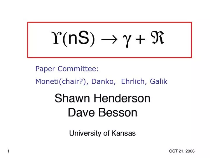
Paper Committee: Moneti(chair?), Danko, Ehrlich, Galik. 1 OCT 21, 2006. History/Bibliography :. Most germane previous CLEO publication: Direct Photon Spectrum from Upsilon(1S),Upsilon(2S) and Upsilon(3S) Decays Phys. Rev. D 74, 012003 (2006)

E N D
Paper Committee: Moneti(chair?), Danko, Ehrlich, Galik 1 OCT 21, 2006
History/Bibliography: Most germane previous CLEO publication: Direct Photon Spectrum from Upsilon(1S),Upsilon(2S) and Upsilon(3S) Decays Phys. Rev. D 74, 012003 (2006) Last plenary presentation by Shawn at Sept. meeting (almost No changes since. Conference paper:Measurement of Upper Limits for Upsilon to gamma + Resonance Decays, J. Rosner et al. Presented at 33rd International Conference on High Energy Physics, July 26- August 2, 2006, Moscow (ICHEP06) hep-ex/0607054 CBX, Draft at http://w4.lns.cornell.edu/restricted/draft/.. Y_GammaRes_CBX.ps( or PDF), Y_GammaRes_PRD.ps( or PDF) Intended for PRD publication 2 OCT 21, 2006
Motivation s extraction in gg analysis: Exp’t and theory assume a continuous direct photon spectrum in determining BR(Y—> gg )/BR(Y—> ggg) • Two-body radiative decays comprise a systematic uncertainty in gg analysis(“bumps” in gamma spectrum!) • This is especially true near the kinematic end-point (x~ 1, low M). We DO see (small) Y—> + f2(1270) • Resonant enhancements could explain why estimates of s from decays are systematically lower than the world average 3 OCT 21, 2006
Look for a Resonance Signal Above suggests a search for + , 4 charged tracks using samehadronic event selection as published ggg analysis. • A two-body radiativedecay will produce a monochromatic in the lab frame, leading to ''bumps'' in the otherwise smooth predictedtheoretical gg spectrum. • Goal: try to determine upper limits on (narrow)resonance contribution to gg rate. • Complication: bkg’d (ISR + hadron fakes) NOT subtracted 4 OCT 21, 2006
MC Example: BIG SIGNAL ! 5 OCT 21, 2006
Brief Analysis Orientation Remember: • XE/Ebeam , M(res) = 2Ebeamsqrt(1- X) For Y(1S), X = 0.2 means M ~ 1 GeV, (E) ~ 20MeV X= 0.9 means M ~ 4.3 GeV, (E) ~ 60MeV We can be largely sensitive to resonances of ~ this width or narrower. Fixed resolution at each X 1) step along X -spectrum in steps of 0.5 (E) , taking a ± 10 range of X X in which to fit for gaussian signal on polynomial background; bin size is 0.2* 2) Extract Area, A(X )of gaussian at each step, plot. 6 OCT 21, 2006
Method (cont.)3) Convert to upper limit contour with height=A(x)+1.645*A(x) where A(x) is the gaussian fit area sigma. 4) Negative points 1.645*A(x)5) Study continuum data, too. Look for evidence of bumps common to Y(nS) and continuum. '' etc…?6) apply estimate (conservative) of efficiency to give BR limits. 7) We use efficiency and 0- (or 0+)1+cos2 for angular distribution.8) re-plot with MR as abcissa 7 OCT 21, 2006
Y(1S) 8 OCT 21, 2006
Y(1S) binned vs. MR 9 OCT 21, 2006
Efficiency corrected BR’s 10 OCT 21, 2006
Y(1S), scaled <Y(1S) comparison Correlated? ISR? 11 OCT 21, 2006
Monte Carlo Check Easy way to check procedure: input known *+, 4 MC signal at various sensitivities and check that which we reconstruct reliably. In this check, we construct all signals above our upper limit floor (~10-4) within our accessible recoil mass range See Plot 12 OCT 21, 2006
MC with 10 embedded R’s if >BR 10-4 then recovered 13 OCT 21, 2006
Result Summary (1) Our sensitivity is of order 10-4 across all accessible values of M • We measure for all M: B((1S)+,4 charged tracks) < 1.26 x 10⁻³ B((2S)+,4 charged tracks) < 9.16 x 10⁻⁴ B((3S)+,4 charged tracks) < 9.69 x 10⁻⁴ B((4S)+,4 charged tracks) < 1.21 x 10⁻³ If more restrictive inM 1.5GeVM 5GeV we do better. 14 OCT 21, 2006
Result Summary (2) B((1S)+,4 charged tracks) < 1.78 x 10⁻⁴ B((2S)+,4 charged tracks) < 1.95 x 10⁻⁴ B((3S)+,4 charged tracks) < 2.20 x 10⁻⁴ B((4S)+,4 charged tracks) < 5.34 x 10⁻⁴ • We report these upper limits as a function of recoiling mass M • B.R.’s are all ~10-4 :unlikely to impact decays in gg analysis 15 OCT 21, 2006
Systematic MattersWe currently assess the following systematics:Exclusive decay channel uncertainty: we take the worst -correction imaginableLuminosity uncertainty: for continuum measurements, we assess a uniform 1% correction (determined in gg analysis)Total # events uncertainty: we take the total number of events to be Nevents() -1eventsSystematic fitting uncertainty: We bin our fitted spectra in 5 bins/signal width and use a 4th order Chebyschev, based on studies of our procedure applied to continuum. Noimpact of polynomial order or binning. 16 OCT 21, 2006
(backup #1) Method (Efficiency Subtleties) • To be conservative, 2 restrictions on the mode we obtain our M-dependent correction function from: • We only consider modes with 4 charged tracks in the final state (should have lowest ’s due to multiplicity cut) • We take as our the worst plausible • We generate 5K events dedicated to each mode, and average the efficiency from 1.0 GeV < E < 4.5 GeV 17 OCT 21, 2006
4 592% 2p2K0 505% 480 602% 4K 502% 22K0 532% 6 743% 4p 672% 420 591% 6K 684% 2p2 623% 4K20 492% 6p 524% 2p2K 562% 4p20 632% 22K 533% 2p220 635% 40 602% 2p2K20 572% 4K0 482% 22K20 543% 4p0 652% 440 572% 2p20 545% 460 602% Efficiencies (*+, →?) Worst Phase Space High Mult. 18 OCT 21, 2006
Worst possible efficiency vs. E 19 OCT 21, 2006