Download
1 / 47
470 likes | 703 Views
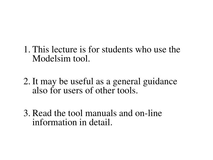
This lecture is for students who use the Modelsim tool. It may be useful as a general guidance also for users of other tools. Read the tool manuals and on-line information in detail. Applications Note 116: VHDL Style Guidelines for Performance. Introduction.

E N D
This lecture is for students who use the Modelsim tool. It may be useful as a general guidance also for users of other tools. Read the tool manuals and on-line information in detail.
Applications Note 116: VHDL Style Guidelines for Performance
Introduction • No matter how fast a simulator gets, the HDL developer can further improve performance by applying a few simple guidelines to the coding style. • The key to higher performance is to avoid code that needlessly creates additional work for the HDL compiler and simulator. • These slides will describe the general code constructs that have a high performance impact, and how to avoid them. • Specifically, we show how to apply the ModelSim Performance Analyzer to improve simulation performance.
Performance Basics • A simulator uses a highly specialized database. • For every event, the simulator must quickly: • find all affected processes, • evaluate these processes, • update the state • and schedule the resulting new events. • As with any database, the more data managed by the simulator the slower the overall transaction time. • The rules below describe the relative performance cost of different VHDL language elements.
Performance Basics • The underlying strategy is to reduce the high cost elements by replacing them with less costly elements or eliminating them entirely. • Obviously, the underlying integrity of the design must be maintained. • The rules below merely describe better ways to implement the same content.
Measuring Performance on UNIX • Accurate performance measurements are necessary when tuning the code. • On UNIX machines you can prefix the vsim invocation using the “time” command. On Solaris this looks like: /usr/bin/time vsim –do perf_test.do . . . real 153.0 user 112.3 sys 4.1 • The “real” line shows how much wall clock time passed. • The “user” line shows how much CPU time was used during the run. • The “sys” line refers to the amount of time taken by operating system calls.
Measuring Performance on UNIX • A large difference between the “real” and “user” time means one of two things: • The system is heavily loaded with other simultaneous processes • The simulation exceeds the memory, and is swapping to disk • Changes to VHDL style are of little help in these cases, as limited computational resources are curtailing simulation performance.
Measuring Performance on NT • On NT machines you can get the same information through the task manager (CTRL-ALT-DEL Task Manager or Right-Click on Task Bar > Task Manager). • Select the Processes tab and find the entry for vsim.exe. • The data CPU time column is cumulative if you run several tests in the same ModelSim session.
Using Performance Analyzer • Here in next slide is a small ModelSim Tcl script that measures wall clock time for a simulation run. • This would be appropriate for a machine that has little running on it besides the simulator. • This script also: • invokes the ModelSim performance analyzer, • opens the report GUI • and writes the performance profile results to a file called “profile.txt”.
TCL script for performance analysis and report writing • Further description of the use of the performance analyzer can be found in the ModelSim documentation and the applications note: “ModelSim HDL Simulation Performance Analyzer”.
HDL Style for Performance • Rule 1: Use Optimized Standard Libraries • Customers report up to a 3x performance increase when switching from unoptimized to optimized VHDL libraries. • For ModelSim, all of the most frequently used VHDL libraries have been specifically tuned for maximum performance within ModelSim. • These optimizations can be disabled by using special switches at compilation (-o0 or –noaccel) or by explicitly mapping in alternate libraries.
HDL Style for Performance • However, the most common reason for poor performance is mistaken use of unoptimized libraries. • This occurs if the build environment compiles standard library source code from a non-Model Tech source. • Source code for standard libraries is often included with synthesis tools or ASIC vendor libraries, and is often compiled by mistake. • These unoptimized librarieswill take precedent over the default ones.
The Performance Analyzer can quickly show you when you are using an unoptimized library. • If the performance report implicates a line within a library (outside of user code) then the library has not been optimized. • Optimized libraries do not show up in the performance analyzer report. • If the library indicated is one in the optimized list of Table 1, then review the steps taken to compile the design. This table shows optimized and unoptimized libraries
Rule 2: Reduce Process Sensitivity • Avoid inefficient processes like this one: inefficient : process (A, B) begin procedure_1(A); procedure_2(B); end process inefficient; • Notice that every time B changes, a call is needlessly made to procedure_1. • Similarly, events on A will force the redundant evaluation procedure_2. • Note that if you have shared data between the two processes, you may have difficulty accurately synthesizing the correct behavior. • In the example above, the Performance Analyzer is likely to identify excess time spent in this process.
Two separate processes, each with the correct sensitivity list is the more efficient coding style: efficient_1 : process (A) begin procedure_1(A); end process efficient_1; efficient_2 : process (B) begin procedure_2(B); end process efficient_2;
This is a trivial example, but processes like these appear often in the customer examples. • Unnecessarily sensitive can severely impact performance. • Also, use caution when creating processes sensitive to signals of record type. • The record may contain more information than the process strictly needs, but any change to any element of the record will force a re-evaluation of the process.
Rule 3: Reducing waits • It is a common practice to use a for looparound a wait on clock to allow a specific amount of time to pass. • This fragment delays 100 clock cycles: for i in 1 to 100 loop wait until Clk’Event and Clk = ‘1’; end loop; next statement ... • While this loop is not complicated, the Performance Analyzer may identify the “wait” line as a bottleneck. • The reason for this is the proliferation of processes waiting for signal events, even though the action taken by each process is minimal.
Although slightly more obscure, the following fragment accomplishes the same behavior: wait for (CLOCK_PERIOD_T * 100 – 1 ns); wait until Clk’Event and Clk = ‘1’; next statement ... • The first fragment schedules 100 process evaluations, while the second requires only two. • The behavior is the same, but the performance consequence is minimized. • The final wait until Clk is needed to ensure proper synchronization with the clock signal. • Without it, the “next statement” is in a unpredictable race condition with whatever is generating the clock.
Rule 4: Reduce or Delay Calculations • The following fragment repeats the same 64-bit calculations at each evaluation of the process: driver : process (Clk) begin if (Clk’event and Clk = ‘1’) then ... D <= Next_D_val after (CLOCK_PERIOD_T – SETUP_T); LD <= Next_LD_val after (CLOCK_PERIOD_T – SETUP_T); ... • The drive times are repeatedly calculated.
With the simple use of a constant, two 64-bit operations per clock cycle are removed: driver : process (Clk) constant DRIVE_T : time := (CLOCK_PERIOD_T – SETUP_T); begin if (Clk’event and Clk = ‘1’) then ... D <= Next_D_val after (DRIVE_T); LD <= Next_LD_val after (DRIVE_T); ...
Another good rule of thumb is to delay calculations until they are needed. Here is an example of an inefficient call to a function: • The example on the left makes the “to_integer” call every evaluation, whether the result is used or not.
Rule 5: Limit File I/O • Reading or writing to files during simulation is costly to performance, because the simulator must halt and wait while the OS completes each transaction with the file system. • Furthermore, the VHDL “read” functions that convert text data to different data types are also costly. • One way to improve performance is to replace ASCII vector fileswith a constant table in VHDL like this one:
One way to improve performance is to use a constant table in VHDL
Advantages of using a constant table in VHDL • The testbench would then loop through each record in the table and drive or check pins appropriately for each clock cycle. • This approach not only removes the file access overhead, no simulation time is spentparsing strings or performing data conversion. • Although the syntax of the vectors above is more complex than a straight ASCII file, it should be easy to generate or translate vector data to this format.
But what are the drawbacks of this table? • One drawback is that the HDL table approach like the example above can cause large compilation times. • Since compilation time grows in a non-linear fashion, at some point the compilation time will exceed the cost of ASCII vectors. • Figure 1 below shows how the number of vectorsaffects total compilation and simulation time with the two approaches.
Figure 1 below shows how the number of vectorsaffects total compilation and simulation time with the two approaches. Compilation time Simulation time
Comparison of simulation and compilation times • For large vector sets, reading and translating the ASCII will edge out HDL vectors when the compilation time is considered. • Simulation performance of HDL vectors will always be better, however. • So, if the HDL vectors are stable, (needing only occasional re-compilation), then HDL vectors will be the better choice. • If file access cannot be eliminated, perhaps it can be reduced.
Comparison of simulation and compilation times • You could read or write more information with each file access, to reduce the overall number. • For example, you could change the format of the input file so that several vectors are contained on each line. • This would reduce the number of calls to “readline”. • Similarly, when writing out data, pack as much as you can into each “writeline” operation. • When using the vsim log or vcd commands, try not to record more information than you really need.
Rule 6: Integers vs. Vectors • Arithmetic operations on Standard Logic Vectors (SLVs) are expensive compared to integer operations. • Consider converting an SLV to an integer, performing the operations and converting the integer back to an SLV. • Integer conversion costs are small compared to costs of even simple SLV operations. • In the example below the unsigned vector “value” is used in a simple comparison (> 0) and a subtraction. • ...if (value > 0) then -- <-- Slowvalue <= value – 1; -- <-- Slowelsevalue <= startValue;end if;...
The performance analyzer might identify the two lines as being the slowest part of this process. • Suppose that for the purposes of your design, two states would suffice for “value”. • You could then use an integer instead:...int_value := to_integer(value);if (int_value > 0) then -- <-- Fastint_value := int_value – 1; -- <-- Fastelseint_value := to_integer(startValue);end if;value <= to_unsigned(int_value, 8);...
How it affects the testbench? • The performance of the process would be significantly improved. • If you have testbench code that generatesonly two-state or four-state behavior, it should be relatively straight-forward to write the testbench using integers instead of std_logic_vectors. • For maximum performance, use ranged integers in entity declarations instead of std_logic_vectors.
Simulator versus synthesis tool • With both the interface and internal state represented in integers, the simulator will be able to process the design much more efficiently. • This is a fairly dramatic step, and you should make sure that your synthesis tools can properly handle ranged integers in your design.
Rule 7: Buffer Clocks Between Mixed HDL • ModelSim is extremely efficient in handling mixed VHDL/Verilog designs. • There is only a slight penalty to move signal events between HDL domains because of the ModelSim single kernel architecture. • If there are hundreds of process in one language domain that are sensitive to a signal in the other domain, the accumulation of this penalty can eventually get large enough to be noticed.
Consider the case where a clock signal generated in VHDL code is connected to a large gate level Verilog design. • In this example, every flip flop in the Verilog design is sensitive to the VHDL generated clock.
Rule 8: Avoid Slicing Signals • If a signal is sliced, vector optimizations cannot be applied. signal A_sig : std_logic_vector (63 downto 0); ... A_sig(3) <= ‘1’; • The signal is probably used in several places in the design. • Even a single bit slice propagates an unoptimized vector to all affected processes.
Wrong and right way of introducting the temporary variable • The introduction of a temporary variable can give you the functionality of a bit slice, without the performance penalty: • In the example on the right, A_sig is kept whole, while the bit slicing occurs for the temporary variable “tmp_A”. • The costs of slicing the temporary variable and the additional assignment are small in comparison to the penalty of an unoptimized signal vector.
Rule 9: Check Optimization of VITAL libraries • During gate level simulation, the profiler may indicate that a small set of primitives are consuming the majority of execution time. • This may be because: • the design have many instances of these primitives, • or that the primitives were not optimized when they were compiled. • Improving a high-use unoptimized cell can help performance significantly. • Determining VITAL Cell Usage • After the design is loaded, use this the write command at the VSIM prompt: write report <filename>
Rule 9: Check Optimization of VITAL libraries • This report will include a list of all entities in the design. • You will have to post process the report with Perl or grep to find the number of instances of the key cells identified by the profiler. • For example grep –c <cell name> <report file> • This will count the number of occurances of the cell name in the report.
Checking VITAL Optimization • Use the -debugVA switch when compiling the design, and save the results to a file: vcom –debugVA MyVitalDesign.vhd > <results file name> • Compile messages and any errors are written to the results_of_compile file. • Search for the string OPT_WHYNOT. grep OPT_WHYNOT <results file name>
Optimization of library cells • The compiler may not be able to optimize a particular Cell for a variety of reasons. • The primitive is based on VITAL 0 instead of VITAL 1. Only VITAL 1 code is optimized. • The Cell contains VITAL non-compliant code • The cell is based on inefficient (usually auto-generated) code • You can submit a bug reportto the library vendor to have the problem fixed. • Many customers are willing to use a copy of the inefficient cell that is hand modified to improve performance. • This optimized cell is used in place of the official one until the final round of validations.
Rule 10: Avoid the “Linear Testbench” • One naïve approach to testbench creation is especially bad for performance. • Here is a fragment of a “linear” testbench:
Drawbacks of this approach • Stimulus code like this is easy to generate (translating a vector file with a Perl script, for example). • However, for a compiled simulator like ModelSim, the simulator must evaluate and schedule a very large number of events. • This reduces simulation performance in proportion to the size of the stimulus process. • As an alternative, consider using the VHDL table approach seen in rule 6 above.
Rule 11: Optimize Everything 0ver 1% • The ModelSim Performance Analyzer will identify the lines of codethat consume the greatest CPU time and display these lines in ranked order in the performance profile window. • Double clicking a line in the report will bring up the source file window with the file and line displayed.
ModelSim Performance Analyzer will identify the lines of code that consume the greatest CPU time • The lines identified by the profiler may not appear to contribute a significant amount to the overall execution time. • Amdahl’s law would suggest that attempting to make 4% of the design run faster could improve overall performance by no more than 4%. • However, making a trivial fix many times reaps a large performance benefit.
making a trivial fix many times reaps a large performance benefit • This is because the change may: • Enable further optimization by the compiler • Reduce the number events • Reduce the number of processes sensitive to events • Thus, a small improvement to the code can have a non-linear result in the overall execution speed. • Optimize any line responsible for more than 1% whenever possible.
Conclusions • With the ModelSim Performance Analyzer, simulation speed is no longer a black box. • Often small changes to a handful of code lines can yield a large performance benefit. • The Performance Analyzer will direct you to the critical performance bottlenecks, and the nine rules above give a general outline as to how to deal with them. • A design and testbench built from scratch using these rules will have maximum performance.