Download

1 / 24
240 likes | 376 Views
PGM: Tirgul 11 Na?ve Bayesian Classifier + Tree Augmented Na?ve Bayes (adapted from tutorial by Nir Friedman and Moises Goldszmidt. Age Sex ChestPain RestBP Cholesterol BloodSugar ECG MaxHeartRt Angina OldPeak Heart Disease. The Classification Problem.

E N D
PGM: Tirgul 11Na?ve Bayesian Classifier +Tree Augmented Na?ve Bayes(adapted from tutorial by Nir Friedman and Moises Goldszmidt
Age Sex ChestPain RestBP Cholesterol BloodSugar ECG MaxHeartRt Angina OldPeak Heart Disease The Classification Problem • From a data set describing objects by vectors of features and a class • Find a function F: featuresclass to classify a new object Vector1= <49, 0, 2, 134, 271, 0, 0, 162, 0, 0, 2, 0, 3> Presence Vector2= <42, 1, 3, 130, 180, 0, 0, 150, 0, 0, 1, 0, 3>Presence Vector3= <39, 0, 3, 94, 199, 0, 0, 179, 0, 0, 1, 0, 3 >Presence Vector4= <41, 1, 2, 135, 203, 0, 0, 132, 0, 0, 2, 0, 6 >Absence Vector5= <56, 1, 3, 130, 256, 1, 2, 142, 1, 0.6, 2, 1, 6 >Absence Vector6= <70, 1, 2, 156, 245, 0, 2, 143, 0, 0, 1, 0, 3 >Presence Vector7= <56, 1, 4, 132, 184, 0, 2, 105, 1, 2.1, 2, 1, 6 >Absence
Examples • Predicting heart disease • Features: cholesterol, chest pain, angina, age, etc. • Class: {present, absent} • Finding lemons in cars • Features: make, brand, miles per gallon, acceleration,etc. • Class: {normal, lemon} • Digit recognition • Features: matrix of pixel descriptors • Class: {1, 2, 3, 4, 5, 6, 7, 8, 9, 0} • Speech recognition • Features: Signal characteristics, language model • Class: {pause/hesitation, retraction}
Approaches • Memory based • Define a distance between samples • Nearest neighbor, support vector machines • Decision surface • Find best partition of the space • CART, decision trees • Generative models • Induce a model and impose a decision rule • Bayesian networks
Generative Models • Bayesian classifiers • Induce a probability describing the data P(A1,…,An,C) • Impose a decision rule. Given a new object < a1,…,an > c = argmaxC P(C = c | a1,…,an) • We have shifted the problem to learning P(A1,…,An,C) • We are learning how to do this efficiently: learn a Bayesian network representation for P(A1,…,An,C)
Optimality of the decision ruleMinimizing the error rate... • Let ci be the true class, and let lj be the class returned by the classifier. • A decision by the classifier is correct if ci=lj, and in error if ci lj. • The error incurred by choose label lj is • Thus, had we had access to P, we minimize error rate by choosing liwhenwhich is the decision rule for the Bayesian classifier
Advantages of the Generative Model Approach • Output: Rank over the outcomes---likelihood of present vs. absent • Explanation: What is the profile of a “typical” person with a heart disease • Missing values: both in training and testing • Value of information: If the person has high cholesterol and blood sugar, which other test should be conducted? • Validation: confidence measures over the model and its parameters • Background knowledge: priors and structure
Partition the data set in n segments Do n times Train the classifier with the green segments Test accuracy on the red segments Compute statistics on the n runs Variance Mean accuracy Accuracy: on test data of size m Acc = Evaluating the performance of a classifier: n-fold cross validation D1 D2 D3 Dn Run 1 Run 2 Run 3 Run n Original data set
Outcome Age MaxHeartRate Vessels STSlope Angina BloodSugar OldPeak ChestPain RestBP ECG Thal Sex Cholesterol Advantages of Using a Bayesian Network • Efficiency in learning and query answering • Combine knowledge engineering and statistical induction • Algorithms for decision making, value of information, diagnosis and repair Heart disease Accuracy = 85% Data source UCI repository
Problems with BNs as classifiers When evaluating a Bayesian network, we examine the likelyhood of the model B given the data D and try to maximize it: When Learning structure we also add penalty for structure complexity and seek a balance between the two terms (MDL or variant). The following properties follow: • A Bayesian network minimized the error over all the variables in the domain and not necessarily the local error of the class given the attributes (OK with enough data). • Because of the penalty, a Bayesian network in effect looks at a small subset of the variables that effect a given node (it’s Markov blanket)
Problems with BNs as classifiers (cont.) Let’s look closely at the likelyhood term: • The first term estimates just what we want: the probability of the class given the attributes. The second term estimates the joint probability of the attributes. • When there are many attributes, the second term starts to dominate (value of log is increased for small values). • Why not use the just the first term? We can no longer factorize and calculations become much harder.
C insulin F1 F2 F3 F4 F5 F6 age mass glucose pregnant dpf The Naïve Bayesian Classifier Diabetes in Pima Indians (from UCI repository) • Fixed structure encoding the assumption that features are independent of each other given the class. • Learning amounts to estimating the parameters for each P(Fi|C) for each Fi.
The Naïve Bayesian Classifier (cont.) What do we gain? • We ensure that in the learned network, the probability P(C|A1…An) will take every attribute into account. • We will show polynomial time algorithm for learning the network. • Estimates are robust consisting of low order statistics requiring few instances • Has proven to be a powerful classifier often exceeding unrestricted Bayesian networks.
C F1 F2 F3 F4 F5 F6 The Naïve Bayesian Classifier (cont.) • Common practice is to estimate • These estimate are identical to MLE for multinomials
Improving Naïve Bayes • Naïve Bayes encodes assumptions of independence that may be unreasonable: Are pregnancy and age independent given diabetes? Problem: same evidence may be incorporated multiple times (a rare Glucose level and a rare Insulin level over penalize the class variable) • The success of naïve Bayes is attributed to • Robust estimation • Decision may be correct even if probabilities are inaccurate • Idea: improve on naïve Bayes by weakening the independence assumptions Bayesian networks provide the appropriate mathematical language for this task
C mass dpf pregnant age glucose F1 F2 F4 F5 F6 insulin F3 Tree Augmented Naïve Bayes (TAN) • Approximate the dependence among features with a tree Bayes net • Tree induction algorithm • Optimality: maximum likelihood tree • Efficiency: polynomial algorithm • Robust parameter estimation
Optimal Tree construction algorithm The procedure of Chow and Lui construct a tree structure BT that maximizes LL(BT |D) • Compute the mutual information between every pair of attributes: • Build a complete undirected graph in which the vertices are the attributes and each edge is annotated with the corresponding mutual information as weight. • Build a maximum weighted spanning tree of this graph. Complexity: O(n2N) + O(n2) + O(n2logn) = O(n2N) where n is the number of attributes and N is the sample size
Tree construction algorithm (cont.) It is easy to “plant” the optimal tree in the TAN by revising the algorithm to use a revised conditional measure which takes the conditional probability on the class into account: This measures the gain in the log-likelyhood of adding Ai as a parent of Aj when C is already a parent.
Problem with TAN When evaluating parameters we estimate the conditional probability P(Ai|Parents(Ai)). This is done by partitionaing the data according to possible values of Parents(Ai). • When a partition contains just a few instances we get an unreliable estimate • In Naive Bayes the partition was only on the values of the classifier (and we have to assume that is adequate) • In TAN we have twice the number of partitions and get unreliable estimates, especially for small data sets. Solution: where s is the smoothing bias and typically small.
Performance: TAN vs. Naïve Bayes 100 • 25 Data sets from UCI repository • Medical • Signal processing • Financial • Games • Accuracy based on 5-fold cross-validation • No parameter tuning 95 90 85 Naïve Bayes 80 75 70 65 65 70 75 80 85 90 95 100 TAN
Performance: TAN vs C4.5 • 25 Data sets from UCI repository • Medical • Signal processing • Financial • Games • Accuracy based on 5-fold cross-validation • No parameter tuning 100 95 90 85 C4.5 80 75 70 65 65 70 75 80 85 90 95 100 TAN
Beyond TAN • Can we do better by learning a more flexible structure? • Experiment: learn a Bayesian network without restrictions on the structure
100 95 90 85 80 75 70 65 65 70 75 80 85 90 95 100 Performance: TAN vs. Bayesian Networks • 25 Data sets from UCI repository • Medical • Signal processing • Financial • Games • Accuracy based on 5-fold cross-validation • No parameter tuning Bayesian Networks TAN
Classification: Summary • Bayesian networks provide a useful language to improve Bayesian classifiers • Lesson: we need to be aware of the task at hand, the amount of training data vs dimensionality of the problem, etc • Additional benefits • Missing values • Compute the tradeoffs involved in finding out feature values • Compute misclassification costs • Recent progress: • Combine generative probabilistic models, such as Bayesian networks, with decision surface approaches such as Support Vector Machines