Download
1 / 36
400 likes | 569 Views
AGE ESTIMATION: A CLASSIFICATION PROBLEM. HANDE ALEMDAR, BERNA ALTINEL, NEŞE ALYÜZ, SERHAN DANİŞ. Project Overview. Subset Overview. Aging Subset of Bosphorus Database: 1-4 neutral and frontal 2D images of subjects 105 subjects Total of 298 scans Age range: [18-60]

E N D
AGE ESTIMATION: A CLASSIFICATION PROBLEM HANDE ALEMDAR, BERNA ALTINEL, NEŞE ALYÜZ, SERHAN DANİŞ
Subset Overview • Aging Subset of Bosphorus Database: • 1-4 neutral and frontal 2D images of subjects • 105 subjects • Total of 298 scans • Age range: [18-60] • Age distribution non uniform: average = 29.9
Project Overview • Aging images of individuals is not present • Aim: Age Estimation based on Age Classes • 3 Classes: • Age<26 -> 96 samples • 26 <= Age <= 35 -> 161 samples • Age>36 -> 41 samples
Preprocessing • Registration • Cropping • Histogram Equalization • Resizing
Neşe Alyüz Subspace analysis for age estimation
Age Manifold • Instead of learning a subject-specific aging pattern, a common aging trend can be learned • Manifold embedding technique to learn the low-dimensional aging trend. Image space: Labels: Low-dim. representation: d<<D Mapping:
Orthogonal Locality Preserving Projections - OLPP • Subspace learning technique • Produces orthogonal basis functions on LPP • LPP: The essential manifold structure preserved by measuring local neighborhood distances • OLPP vs. PCA for age manifold: • OLPP is supervised, PCA is unsupervised • OLPP better, since age labeling is used for learning X Size of training data for OLPP should be LARGE enough
Locality Preserving Projection - LPP • aka: Laplacianface Approach • Linear dimensionality reduction algorithm • Builds a graph: based on neighborhood information • Obtains a linear transformation: Neighborhood information is preserved
LPP • S: similarity matrix defined on data points (weights) • L = D – S : graph Laplacian • D: diagonal sum matrix of S measures local density around a sample point • Minimization problem: with the constraint : => Minimizing this function: ensure that if xi and xj are close then their projections yi and yj are also close
LPP • Generalized eigenvalue problem: • Basis functions are the eigenvectors of: Not symmetric, therefore the basis functions are not orthogonal
OLPP • In LPP, basis functions are nonorthogonal • > reconstruction is difficult • OLPP produces orthogonal basis functions • > has more locality preserving power
OLPP – Algorithmic Outline (1) Preprocessing: PCA projection (2) Constructing the Adjacency Graph (3) Choosing the Locality Weights (4) Computing the Orthogonal Basis Functions (5) OLPP Embedding
(1) Preprocessing: PCA Prjection • XDXT can be singular • To overcome the singularity problem -> PCA • Throwing away components, whose corresponding eigenvalues are zero. • Transformation matrix: WPCA • Extracted features become statistically uncorrelated
(2) Constructing The Adjacency Graph • G: a graph with n nodes • If face images xi and xj are connected (has the same label) then an edge exists in-between.
(3) Choosing the Locality Weights • S: weight matrix • If node i and j are connected: • Weights: heat kernel function • Models the local structure of the manifold
(4) Computing the Orthogonal Basis Functions • D: diagonal matrix, column sum of S • L : laplacian matrix, L = D – S • Orthogonal basis vectors: • Two extra matrices defined: • Computing the basis vectors: • Compute a1 : eigenvector of with the greatest eigenvalue • Compute ak : eigenvector of with the greatest eigenvalue
(5) OLPP Embedding • Let: • Overall embedding:
Subspace Methods: PCA vs. OLPP • Face Recognition Results on ORL
Subspace Methods: PCA vs. OLPP • Face Recognition Results on Aging Subset of the Bosphorus Database • Age Estimation (Classification) Results on Aging Subset of the Bosphorus Database
Hande Alemdar Feature extraction: Local binary patterns
Feature Extraction • LBP - Local Binary Patterns
Local Binary Patterns • More formally • For 3x3 neighborhood we have 256 patterns • Feature vector size = 256 where
Uniform LBP • Uniform patternscan be used to reduce the length of the feature vector and implement a simple rotation-invariant descriptor • If the binary pattern contains at most two bitwise transitions from 0 to 1 or vice versa when the bit pattern is traversed circularly Uniform • 01110000 is uniform • 00111000 (2 transitions) • 00011100 (2 transitions) • For 3x3 neighborhood we have 58 uniform patterns • Feature vector size = 59
Serhan Daniş Feature extraction: Gabor Filtering
Gabor Filter • Band-pass filters used for feature extraction, texture analysis and stereo disparity estimation. • Can be designed for a number of dilations and rotations. • The filters with various dilations and rotations are convolved with the signal, resulting in a so-called Gabor space. This process is closely related to processes in the primary visual cortex.
A set of Gabor filters with different frequencies and orientations may be helpful for extracting useful features from an image. We used 6 different rotations and 4 different scales on 16 overlapping patches of the images. We generate 768 features for each image. Gabor Filter
Berna Altınel Classification
EXPERIMENTAL DATASETS 1. Features_50_45(LBP) 2. Features_100_90(LBP)3. Features_ORIg(LBP)4. Features_50_45(GABOR)5. Features_100_90 (GABOR)
Experiment #1 Estimate age, just based on the average value of the training set
The K-nearest-neighbor (KNN) algorithm measures the distance between a query scenario and a set of scenarios in the data set. Experiments #2 K-nearest-neighbor algorithm
[2 [2 1. Parametric Classification 2. Mahalanobis distance can be used as the distance measure in kNN. IN PROGRESS:
1. Other distance functions can be analyzed for kNN: 2. Normalization can be applied: POSSIBLE FUTURE WORK ITEMS: