Download
1 / 29
290 likes | 306 Views
Methods for Solution of the System of Equations: Ax = b Direct Methods: one obtains the exact solution (ignoring the round-off errors) in a finite number of steps. These group of methods are more efficient for dense and banded matrices. Gauss Elimination; Gauss-Jordon Elimination

E N D
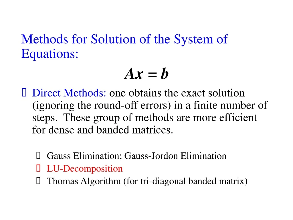
Methods for Solution of the System of Equations: Ax = b • Direct Methods: one obtains the exact solution (ignoring the round-off errors) in a finite number of steps. These group of methods are more efficient for dense and banded matrices. • Gauss Elimination; Gauss-Jordon Elimination • LU-Decomposition • Thomas Algorithm (for tri-diagonal banded matrix)
LU-Decomposition: A general method Ax = b • In most engineering problems, the matrix A remains constant while the vector b changes with time. The matrix A describes the system and the vector b describes the external forcing. e.g., all network problems (pipes, electrical, canal, road, reactors, etc.); structural frames; many financial analyses. • If all b’s are available together, one can solve the system by augmented matrix but in practice, they are not! • Instead of performing ⁓ n3 floating point operations to solve whenever a new b becomes available, it is possible to solve the system by performing ⁓ n2 floating point operations if a LU Decomposition is available for matrix A • LU-decomposition requires ⁓ n3 floating point operations!
Consider the system: (b changes!) Ax = b • Perform a decomposition of the form A = LU, where L is a lower-triangular and U is an upper-triangular matrix! • LU-decomposition requires ⁓ n3 floating point operations! • For any given b, solve Ax = LUx = b • This is equivalent to solving two triangular systems: • Solve Ly = b using forward substitution to obtain y (~n2 operations) • Solve Ux = y using back substitution to obtain x (~n2 operations) • Most frequently used method for engineering applications! • We will derive LU-decomposition from Gauss Elimination!
Define the elements of matrix L as: • Define the elements of matrix U as: Any element aij is actively modified for the first p steps • This is equivalent to matrix multiplication: A = LU
12 Unknowns and 9 equations! 3 free entries! In general, n2 equations and n2 + n unknows! n free entries!
Doolittle’s Algorithm: Define: • The U matrix: i ≤ j • The L matrix: j <i
Crout’s Algorithm: Define: • The L matrix: j ≤i • The U matrix: i < j
2 4 Doolittle’s Algorithm (3×3 example): • The L matrix: j <i • j = 1, i = 2, 3: , • j = 2, i = 3: • The U matrix: i ≤ j • i = 1, j = 1, 2, 3: • i = 2, j = 2, 3: • i = 3, j = 3: 1 3 5
1 3 5 Crout’s Algorithm (3×3 example): Define: • The L matrix: j ≤i • The U matrix: i < j Verify this computation sequence! 2 4
LU Theorem: Let Ak be a sequence of matrices formed by first k rows and k columns of a n × n square matrix A. If det (Ak) ≠ 0 for k = 1, 2, … (n-1), then there exist an upper triangular matrix U and a lower triangular matrix L such that, A = LU. Furthermore, if the diagonal elements of either L or U are unity, i.e. lii or uii = 1 for i = 1,2, … n, both L and U are unique. A = Ak = Ak For k = 1, the theorem is trivially valid! b Ak-1 Let’s assume that, the theorem is valid for (k - 1) and prove it for k cT
Ak = LkUk • Lk-1Uk-1 = Ak-1: exists uniquely (by assumption). Also note that the following is valid, det(Ak-1) = det(Lk-1).det(Uk-1) ≠ 0 • Lk-1u = b : Since det(Lk-1) ≠ 0, the triangular system has a unique solution for the vector u • lTUk-1 = cTor Uk-1Tl = c: Since det(Uk-1) ≠ 0, the triangular system has a unique solution for the vector l • lTu + ukk = akk : Since l and u are unique, ukk is unique. Condition for existence: det(Ak-1) = det(Lk-1).det(Uk-1) ≠ 0
Diagonalization (LDU theorem): Let A be a n × n invertible matrix then there exists a decomposition of the form A = LDU where, L is a n × n lower triangular matrix with diagonal elements as 1, U is a n × n upper triangular matrix with diagonal elements as 1, and D is a n × n diagonal matrix. (Can you prove it? also done in MTH 102) Example of a 3 × 3 matrix: For symmetric matrix: U = LT and A = LDLT Note that the entries of the diagonal matrix D are the pivots!
For positive definite matrices, pivots are positive! • Therefore, a diagonal matrix D containing the pivots can be factorized as: D = D1/2D1/2 • Example of a 3 × 3 matrix • For positive definitematrices: A = LDLT = L D1/2D1/2 LT • However, D1/2LT = (LD1/2)T. Denote: L D1/2 = L1 • Therefore, A = L1 L1T . This is also a LU-Decomposition where one needs to evaluate only one triangular matrix L1.
Cholesky Algorithm (for symmetric positive definite matrices): A = LLT .where U = LT. Elements of matrix L are to be evaluated! • Diagonal elements of the L matrix: j =i = p, ljk = ukj • Off-diagonal elements of the L matrix: j < i, p = j, ljk = ukj
A is a positive definite matrix. • This implies:- • A is a symmetric matrix, A = AT • For any non-zero column vector x of n real numbers, xTAx > 0 • Hence, it can be decomposed into LLT by Cholesky algorithm CholeskyAlgorithm: Example Problem
Solve for coefficients of the L matrix, column by column (increasing j) CholeskyAlgorithm: Example Problem • Diagonal elements of the L matrix: • Off-diagonal elements of the L matrix: j < i,
If you already have a LU-decomposition available for matrix A: • Can you use it to compute the inverse? • Can you use it compute the determinant?
Banded Matrix Band Width = a + b - 1 A system of equation with Tri-diagonal coefficient matrix. Total number of elements = n2. Non-zero elements = 3n-2
Tri-Diagonal Matrix: Origin Solution of differential equations of the form: Interpolation, such as by cubic splines:
Thomas Algorithm (for Tridiagonal) • No need to store n2 + n elements! • Store only 4n elements in the form of four vectors l, d, u and b • ith equation is: • Notice: l1 = un = 0
Thomas Algorithm • Initialize two new vectors α and βas α1 = d1and β1 = b1 • Take the first two equations and eliminate x1 : • Resulting equation is: where, • Similarly, we can eliminate x2, x3 ……
Thomas Algorithm • At the ith step: • Eliminate xi-1 to obtain: where,
Thomas Algorithm • Last two equations are: • Eliminate xn-1 to obtain:
Thomas Algorithm • Given: four vectors l, d, u and b • Generate: two vectors α and βas α1 = d1and β1 = b1 i = 2, 3, ….. n • Solution: i = n-1 …… 3, 2, 1 • FP operations: 8(n-1) + 3(n-1) + 1 = 11n - 10


