Download
1 / 72
720 likes | 1.04k Views
Problem Solving. Russell and Norvig: Chapter 3 CSMSC 421 – Fall 2005. sensors. environment. ?. agent. actuators. Problem-Solving Agent. sensors. environment. ?. agent. actuators. Formulate Goal Formulate Problem States Actions Find Solution. Problem-Solving Agent.

E N D
Problem Solving Russell and Norvig: Chapter 3 CSMSC 421 – Fall 2005
sensors environment ? agent actuators Problem-Solving Agent
sensors environment ? agent actuators • Formulate Goal • Formulate Problem • States • Actions • Find Solution Problem-Solving Agent
Holiday Planning • On holiday in Romania; Currently in Arad. Flight leaves tomorrow from Bucharest. • Formulate Goal: Be in Bucharest • Formulate Problem: States: various cities Actions: drive between cities • Find solution: Sequence of cities: Arad, Sibiu, Fagaras, Bucharest
States Actions Solution Goal Start Problem Formulation
Search Problem • State space • each state is an abstract representation of the environment • the state space is discrete • Initial state • Successor function • Goal test • Path cost
Search Problem • State space • Initial state: • usually the current state • sometimes one or several hypothetical states (“what if …”) • Successor function • Goal test • Path cost
Search Problem • State space • Initial state • Successor function: • [state subset of states] • an abstract representation of the possible actions • Goal test • Path cost
Search Problem • State space • Initial state • Successor function • Goal test: • usually a condition • sometimes the description of a state • Path cost
Search Problem • State space • Initial state • Successor function • Goal test • Path cost: • [path positive number] • usually, path cost = sum of step costs • e.g., number of moves of the empty tile
8 2 1 2 3 3 4 7 4 5 6 5 1 6 7 8 Initial state Goal state Example: 8-puzzle
8 2 8 2 7 3 4 7 3 4 5 1 6 5 1 6 8 2 8 2 3 4 7 3 4 7 5 1 6 5 1 6 Example: 8-puzzle
0.18 sec 6 days 12 billion years 10 million states/sec Example: 8-puzzle Size of the state space = 9!/2 = 181,440 15-puzzle .65 x1012 24-puzzle .5 x1025
Example: 8-queens Place 8 queens in a chessboard so that no two queens are in the same row, column, or diagonal. A solution Not a solution
Example: 8-queens • Formulation #1: • States: any arrangement of • 0 to 8 queens on the board • Initial state: 0 queens on the • board • Successor function: add a • queen in any square • Goal test: 8 queens on the • board, none attacked 648 states with 8 queens
Example: 8-queens • Formulation #2: • States: any arrangement of • k = 0 to 8 queens in the k • leftmost columns with none • attacked • Initial state: 0 queens on the • board • Successor function: add a • queen to any square in the leftmost empty column such that it is not attacked • by any other queen • Goal test: 8 queens on the • board 2,067 states
Example: Robot navigation What is the state space?
Cost of one horizontal/vertical step = 1 Cost of one diagonal step = 2 Example: Robot navigation
Complex function: it must find if a collision-free merging motion exists • Successor function: • Merge two subassemblies Example: Assembly Planning Initial state Goal state
Assumptions in Basic Search • The environment is static • The environment is discretizable • The environment is observable • The actions are deterministic
Simple Agent Algorithm Problem-Solving-Agent • initial-state sense/read state • goal select/read goal • successor select/read action models • problem (initial-state, goal, successor) • solution search(problem) • perform(solution)
Search of State Space search tree
Basic Search Concepts • Search tree • Search node • Node expansion • Search strategy: At each stage it determines which node to expand
8 8 2 2 8 2 7 3 3 4 4 7 7 3 4 5 5 1 1 6 6 5 1 6 8 2 3 4 7 8 4 8 2 2 3 4 7 3 7 5 1 6 5 1 6 5 1 6 Search Nodes States The search tree may be infinite even when the state space is finite
Node Data Structure • STATE • PARENT • ACTION • COST • DEPTH If a state is too large, it may be preferable to only represent the initial state and (re-)generate the other states when needed
Fringe • Set of search nodes that have not been expanded yet • Implemented as a queue FRINGE • INSERT(node,FRINGE) • REMOVE(FRINGE) • The ordering of the nodes in FRINGE defines the search strategy
Search Algorithm • If GOAL?(initial-state) then return initial-state • INSERT(initial-node,FRINGE) • Repeat: • If FRINGE is empty then return failure • n REMOVE(FRINGE) • s STATE(n) • For every state s’ in SUCCESSORS(s) • Create a node n’ • If GOAL?(s’) then return path or goal state • INSERT(n’,FRINGE)
Search Strategies • A strategy is defined by picking the order of node expansion • Performance Measures: • Completeness – does it always find a solution if one exists? • Time complexity – number of nodes generated/expanded • Space complexity – maximum number of nodes in memory • Optimality – does it always find a least-cost solution • Time and space complexity are measured in terms of • b – maximum branching factor of the search tree • d – depth of the least-cost solution • m – maximum depth of the state space (may be ∞)
Remark • Some problems formulated as search problems are NP-hard problems. We cannot expect to solve such a problem in less than exponential time in the worst-case • But we can nevertheless strive to solve as many instances of the problem as possible
Blind vs. Heuristic Strategies • Blind (or uninformed) strategies do not exploit any of the information contained in a state • Heuristic (or informed) strategies exploits such information to assess that one node is “more promising” than another
Blind Search… • …[the ant] knew that a certain arrangement had to be made, but it could not figure out how to make it. It was like a man with a tea-cup in one hand and a sandwich in the other, who wants to light a cigarette with a match. But, where the man would invent the idea of putting down the cup and sandwich—before picking up the cigarette and the match—this ant would have put down the sandwich and picked up the match, then it would have been down with the match and up with the cigarette, then down with the cigarette and up with the sandwich, then down with the cup and up with the cigarette, until finally it had put down the sandwich and picked up the match. It was inclined to rely on a series of accidents to achieve its object. It was patient and did not think… Wart watched the arrangements with a surprise which turned into vexation and then into dislike. He felt like asking why it did not think things out in advance… T.H. White, The Once and Future King
Step cost = 1 Step cost = c(action) > 0 Blind Strategies • Breadth-first • Bidirectional • Depth-first • Depth-limited • Iterative deepening • Uniform-Cost
1 2 3 4 5 6 7 Breadth-First Strategy New nodes are inserted at the end of FRINGE FRINGE = (1)
1 2 3 4 5 6 7 Breadth-First Strategy New nodes are inserted at the end of FRINGE FRINGE = (2, 3)
1 2 3 4 5 6 7 Breadth-First Strategy New nodes are inserted at the end of FRINGE FRINGE = (3, 4, 5)
1 2 3 4 5 6 7 Breadth-First Strategy New nodes are inserted at the end of FRINGE FRINGE = (4, 5, 6, 7)
Evaluation • b: branching factor • d: depth of shallowest goal node • Complete • Optimal if step cost is 1 • Number of nodes generated:1 + b + b2 + … + bd + b(bd-1) = O(bd+1) • Time and space complexity is O(bd+1)
Time and Memory Requirements Assumptions: b = 10; 1,000,000 nodes/sec; 100bytes/node
Time and Memory Requirements Assumptions: b = 10; 1,000,000 nodes/sec; 100bytes/node
Bidirectional Strategy 2 fringe queues: FRINGE1 and FRINGE2 Time and space complexity =O(bd/2)<<O(bd)