Download
1 / 22
220 likes | 370 Views
Predicting the performance of climate predictions Chris Ferro (University of Exeter) Tom Fricker , Fredi Otto, Emma Suckling. 13th EMS Annual Meeting and 11th ECAM (10 September 2013, Reading, UK). Performance-based arguments.

E N D
Predicting the performance of climate predictions Chris Ferro (University of Exeter) Tom Fricker, Fredi Otto, Emma Suckling 13th EMS Annual Meeting and 11th ECAM (10 September 2013, Reading, UK)
Performance-based arguments Extrapolate past performance on basis of knowledge of the climate model and the real climate (Parker 2010). Define a reference class of predictions (including the prediction in question) whose performances you cannot reasonably order in advance, measure the performance of some members of the class, and infer the performance of the prediction in question. Popular for weather forecasts (many similar forecasts) but less use for climate predictions (Frame et al. 2007).
Bounding arguments 1. Form a reference class of predictions that does not contain the prediction in question. 2. Judge if the prediction in question is a harder or easier problem than those in the reference class. 3. Measure the performance of some members of the reference class. This bounds your expectations about the performance of the prediction in question (Otto et al. 2013).
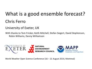
Hindcast example Global mean, annual mean surface air temperature anomalies relative to mean over the previous 20 years. Initial-condition ensembles of HadCM3 launched every year from 1960 to 2000. Measure performance by the absolute errors and consider a lead time of 9 years. 1. Perfect model: predict another HadCM3 member 2. Imperfect model: predict a MIROC5 member 3. Reality: predict HadCRUT4 observations
Recommendations Use existing data explicitly to justify quantitative predictions of the performance of climate predictions. Collect data on more predictions, covering a range of physical processes and conditions, to tighten bounds. Design hindcasts and imperfect model experiments to be as similar as possible to future prediction problems. Train ourselves to be better judges of relative performance, especially to avoid over-confidence.
References Ferro CAT (2013) Fair scores for ensemble forecasts. Submitted Frame DJ, Faull NE, Joshi MM, Allen MR (2007) Probabilistic climate forecasts and inductive problems. Philos. Trans. R. Soc. A 365, 1971-1992 Fricker TE, Ferro CAT, Stephenson DB (2013) Three recommendations for evaluating climate predictions. Meteorol. Appl. 20, 246-255 Goddard L, co-authors (2013) A verification framework for interannual-to-decadal predictions experiments. Clim. Dyn. 40, 245-272 Otto FEL, Ferro CAT, Fricker TE, Suckling EB (2013) On judging the credibility of climate predictions. Clim. Change, in press Parker WS (2010) Predicting weather and climate: uncertainty, ensembles and probability. Stud. Hist. Philos. Mod. Phys. 41, 263-272
Bounding arguments S = performance of a prediction from reference class C S′ = performance of the prediction in question, from C′ Let performance be positive with smaller values better. Infer probabilities Pr(S > s) from a sample from class C. If C′ is harder than C then Pr(S′ > s) > Pr(S > s) for all s. If C′ is easier than C then Pr(S′ > s) < Pr(S > s) for all s.
Future developments Bounding arguments may help us to form fully probabilistic judgments about performance. Let s = (s1, ..., sn) be a sample from S ~ F(∙|p). Let S′ ~ F(∙|cp) with priors p ~ g(∙) and c ~ h(∙). Then Pr(S′ ≤ s|s) = ∫∫F(s|cp)h(c)g(p|s)dcdp. Bounding arguments refer to prior beliefs about S′ directly rather than indirectly through beliefs about c.
Evaluating climate predictions 1. Large trends over the verification period can inflate spuriously the value of some verification measures, e.g. correlation. Scores, which measure the performance of each forecast separately before averaging, are immune to spurious skill. Correlation: 0.06 and 0.84
Evaluating climate predictions 2. Long-range predictions of short-lived quantities (e.g. daily temperatures) can be well calibrated, and may exhibit resolution. Evaluate predictions for relevant quantities, not only multi-year means.
Evaluating climate predictions n = 2 3. Scores should favour ensembles whose members behave as if they and the observation are sampled from the same distribution. ‘Fair’ scores do this; traditional scores do not. unfair score fair score n = 4 n = 8 Figure: The unfair continuous ranked probability score is optimized by under-dispersed ensembles of size n.
Summary Use existing data explicitly to justify quantitative predictions of the performance of climate predictions. Be aware that some measures of performance may be inflated spuriously by climate trends. Consider climate predictions of more decision-relevant quantities, not only multi-year means. Use fair scores to evaluate ensemble forecasts.
Fair scores for ensemble forecasts Let s(p,y) be a scoring rule for a probability forecast, p, and observation, y. The rule is proper if its expectation, Ey[s(p,y)], is optimized when y ~ p. No forecasts score better, on average, than the observation’s distribution. Let s(x,y) be a scoring rule for an ensemble forecast, x, sampled randomly from p. The rule is fair if Ex,y[s(x,y)] is optimized when y ~ p. No ensembles score better, on average, than those from the observation’s distribution. Fricker et al. (2013), Ferro (2013)
Fair scores: binary characterization Let y = 1 if an event occurs, and let y = 0 otherwise. Let si,y be the (finite) score when i of n ensemble members forecast the event and the observation is y. The (negatively oriented) score is fair if (n – i)(si+1,0 – si,0) = i(si-1,1 – si,1) for i = 0, 1, ..., n and si+1,0 ≥ si,0 for i = 0, 1, ..., n – 1. Ferro (2013)
Fair scores: example The (unfair) ensemble version of the continuous ranked probability score is where pn(t) is the proportion of the n ensemble members (x1, ..., xn) no larger than t, and where I(A) = 1 if A is true and I(A) = 0 otherwise. A fair version is
Fair scores: example n = 2 Unfair (dashed) and fair (solid) expected scores against σ when y ~ N(0,1) and xi ~ N(0,σ2) for i = 1, ..., n. n = 4 n = 8
Predicting performance We might try to predict performance by forming our own prediction of the predictand. If we incorporate information about the prediction in question then we must already have judged its credibility; if not then we ignore relevant information. Consider predicting a coin toss. Our own prediction is Pr(head) = 0.5. Then our prediction of the performance of another prediction is bound to be Pr(correct) = 0.5 regardless of other information about that prediction.