Download
1 / 40
410 likes | 564 Views
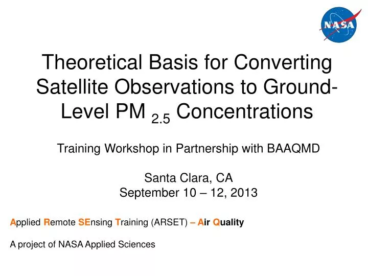
Theoretical Basis for Converting Satellite Observations t o Ground-Level PM 2.5 Concentrations. Training Workshop in Partnership with BAAQMD Santa Clara, CA September 10 – 12, 2013. A pplied R emote SE nsing T raining (ARSET) – A ir Q uality A project of NASA Applied Sciences.

E N D
Theoretical Basis for Converting Satellite Observations to Ground-Level PM 2.5 Concentrations Training Workshop in Partnership with BAAQMD Santa Clara, CASeptember 10 – 12, 2013 Applied Remote SEnsingTraining (ARSET)–Air Quality A project of NASA Applied Sciences
Objective OBJECTIVE Estimate ground-levelPM2.5 mass concentration (µg m-3) using satellite derived AOD
Index Values Category Cautionary Statements PM2.5 (ug/m3) PM10 (ug/m3) 0-50 Good None 0-15.4 0-54 51-100 Moderate Unusually sensitive people should consider reducing prolonged or heavy exertion 15.5-40.4 55-154 101-150 Unhealthy for Sensitive Groups Sensitive groups should reduce prolonged or heavy exertion 40.5-65.4 155-254 151-200 Unhealthy Sensitive groups should avoid prolonged or heavy exertion; everyone else should reduce prolonged or heavy exertion 65.5-150.4 255-354 201-300 Very Unhealthy Sensitive groups should avoid all physical activity outdoors; everyone else should avoid prolonged or heavy exertion 150.5-250.4 355-424 What are we looking for?
What Do Satellites Provide? Satellite Sun Column Satellite Measurement Ozone Rayleigh Scattering 10km Water vapor + other gases (absorption) Seven MODIS bands are utilized to derive aerosol properties: 0.47, 0.55, 0.65, 0.86, 1.24, 1.64, and 2.13µm 10X10 km2 Res. Aerosol Surface Satellite retrieval issues - inversion (e.g. aerosol model, background).
Measurement Techniques AOD – Column integrated value (top of the atmosphere to surface) - Optical measurement of aerosol loading – unitless. AOD is a function of shape, size, type and number concentration of aerosols PM2.5 – Mass per unit volume of aerosol particles less than 2.5 µm in aerodynamic diameter at surface (measurement height) level
May 11, 2007 May 12, 2007 May 13, 2007 May 14, 2007 May 15, 2007 May 16, 2007 MODIS-Terra True Color Images
May 11, 2007 May 12, 2007 May 13, 2007 May 14, 2007 May 15, 2007 May 16, 2007 MODIS-Terra AOD
AOD – PM Relation Composition Size distribution Vertical profile – particle density Q – extinction coefficient re – effective radius fPBL – % AOD in PBL HPBL – mixing height
Support for AOD-PM2.5 Linkage 2 4 6 8 10 12 Current satellite AOD is sensitive to PM2.5(Kahn et al. 1998) Polar-orbiting satellites can represent at least daytime average aerosol loadings (Kaufman et al., 2000) Missing data due to cloud cover appear random in general (Christopher et al., 2010)
Assumption for Quantitative Analysis When most particles are concentrated and well mixed in the boundary layer, satellite AOD contains a strong signal of ground-level particle concentrations.
Modeling the Association of AOD With PM2.5 • The relationship between AOD and PM2.5 depends on parameters hard to measure: • Vertical profile • Size distribution and composition • Diurnal variability • We develop statistical models with variables to represent these parameters • Model simulated vertical profile • Meteorological & other surrogates • Average of multiple AOD measurements No textbook solution!
Methods Developed So Far • Statistical models • Correlation & simple linear regression • Multiple linear regression with effect modifiers • Linear mixed effects models • Geographically weighted regression • Generalized additive models • Hierarchical models combining the above • Bayesian models • Artificial neural network • Data fusion models • Combining satellite data with model simulations • Deterministic models • Improving model simulation with satellite data
Simple Models from Early Days Chu et al., 2003 Wang et al., 2003 13
AOT-PM2.5 Relationship Gupta, 2008
Limitation: Major Unsolved Issue All three Statistical models (TVM, MVM, ANN) underestimate high PM2.5 loadings
Engel-Cox et al., 2006 Al-Saadi et al., 2008 Vertical Distribution
Aug 17 Aug 18 Aug 19 Aug 20 Aug 21 Aug 25 Aug 22 5 km Aug 28 Aug 23 What Satellites can provide for vertical information? - CALIPSO (courtesy of Dave Winker, P.I. CALIPSO)
Advantages of using reanalysis meteorology along with satellite TVM MVM
TVM ANN MVM MODIS-Terra, July 1, 2007 Spatial Comparison • Satellite-derived PM2.5 fills the gap in surface measurements • All three methods underestimate the higher PM2.5 concentrations.
Questions to Ask: Issues • How accurate are these estimates ? • Is the PM2.5-AOD relationship always linear? • How does AOD retrieval uncertainty affect estimation of air quality • Does this relationship change in space and time? • Does this relationship change with aerosol type? • How does meteorology drive this relationship? • How does vertical distribution of aerosols in the atmosphere affect these estimates?
Exposure Modeling Approach Basic idea: PM2.5 = f(AOD, meteorological variables, land use variables, etc.) + ε Census / traffic data land use MODIS AOD NLDAS meteorology Statistical prediction model EPA air monitors Predicted PM2.5 surface
Requirements for this job • PCs with large hard drives and good graphics card • Internet to access satellite & other data • Some statistical software (SAS, R, Matlab, etc.) • Some programming skill • Knowledge of regional air pollution patterns • Ideally, GIS software and working knowledge
Scaling approach Satellite-derived PM2.5= x satellite AOD Basic idea: let an atmospheric chemistry model decide the conversion from AOD to PM2.5. Satellite AOD is used to calibrate the absolute value of the model-generated conversion ratio.
Scaling approach can be applied wherever there are satellite retrievals, but prediction accuracy can vary a lot.
Comparison of two approaches Statistical model Scaling model Mathematically more elegant Applicable in areas with extensive ground data support Requires ability to conduct CTM runs Resolution of predictions dependant on satellite data Lower accuracy (no error terms allowed in the model) • Flexible modeling structure • Ability to provide estimates at high spatial resolution with the help of other covariates • Higher accuracy • Requires extensive ground data support • Models are often not generalizable to other regions
Study Domain Design • Number of monitoring sites: 119 • Exposure modeling domain: 700 x 700 km2
Geographically Weighted Regression Model GWR allows model parameters to vary in space to better capture spatially varying AOD-PM relationship – major advantage over global regression models. Model Structure Datasets (2003): PM2.5 – EPA / IMPROVE daily measurements AOD – MODIS collection 5 (10 km) Meteorology – NLDAS-2 (14 km) Land use: NLCD 2001
Summary Statistics PM2.5 (ug/m3) PBL (m) RH (%) TMP (K)
U-Wind (m/sec) V-Wind (m/sec) Forest (%) AOD
Model Fitting Results Local R2 values vary in time – daily model is necessary. No residual spatial autocorrelation was found in 78% of the daily GWR models. >=10 matched data records is needed to stabilize the model
Model Performance Evaluation Putting all the data points together, we see unbiased estimates Model CV
Spatial Pattern of Model Bias Model Fitting Cross Validation Negative and positive model / CV residuals are randomly distributed.
Model Predicted Mean PM2.5 Surface Note: annual mean calculated with137 days
Comparison with CMAQ General patterns agree, details differ
Caveats MODIS GOES • Data coverage • MISR has the least coverage
Data Quality - MISR urban biomass burning dusty r = 0.92, mean absolute diff = 26% r = 0.87, mean absolute diff = 51% r = 0.93, mean absolute diff = 32% Source: Kahn et al. 2010 Source: Liu et al. 2004 Expected error globally: ±(0.05 or 0.20t) In the US: ±(0.05 or 0.15t)
Data Quality – MODIS DDV Product Expected error: ±(0.05+0.15t) Source: Levy et al. 2010
Data Quality - GOES r = 0.79 over 10 northeastern sites, slope = 0.8 Source: Prados et al. 2007
The Use of Satellite Models • Currently for research • Spatial trends of PM2.5 at regional to national level • Interannual variability of PM2.5 • Model calibration / validation • Exposure assessment for health effect studies • In the near future for research • Spatial trends at urban scale • Improved coverage and accuracy • Fused statistical – deterministic models • For regulation?