Download
1 / 36
360 likes | 496 Views
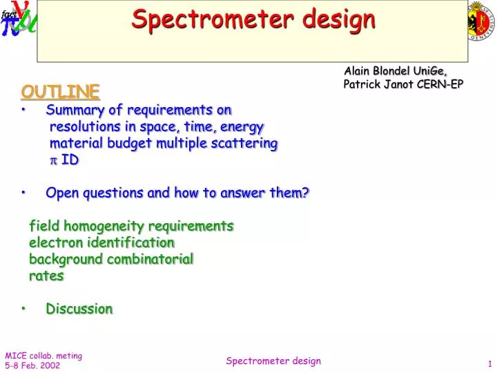
Spectrometer design . Alain Blondel UniGe, Patrick Janot CERN-EP. OUTLINE Summary of requirements on resolutions in space, time, energy material budget multiple scattering ID Open questions and how to answer them? field homogeneity requirements

E N D
Spectrometer design Alain Blondel UniGe, Patrick Janot CERN-EP • OUTLINE • Summary of requirements on • resolutions in space, time, energy • material budget multiple scattering • ID • Open questions and how to answer them? • field homogeneity requirements • electron identification • background combinatorial • rates • Discussion Spectrometer design
Cooling box Tracking devices: Measurement of momentum angles and position Tracking devices T.O.F. III Precise timing T.O.F. I & II Pion /muon ID and precise timing Electron ID Eliminate muons that decay Spectrometer design
DWARF4.0 What’s in it? • Particle transport in magnetic field and in RF; homogeneous field. • Multiple Scattering in matter; • tracker: 4 sets of three layers of 500 micron scintillating fibers • Energy Loss (average and Landau fluctuations) in matter; • Bremsstrahlung in matter; no showering • Beam contamination with pions, pion decay in flight; • Muon decay in flight (with any polarization), electron transport; • Poor-Man Cooling Simulation (only Bz and EZ) to quantify particle and correlation losses with cooling; • Gaussian errors on measured quantities (x, y, t). Spectrometer design
tracking detectors simulated Spectrometer design
DWARF4.0: What’s not in ? • Imperfections of magnetic fields; heating at solenoid exits; (A field map and step tracking will be needed here… Might be the source of important bias and systematic uncertainty • Dead channels; • Misalignment of detector elements; • Background of any origin (RF, beam, …) (Could well spoil the measurement. Need redundancy in case…) • track fit in presence of noise and dead channels (pattern recognition) • electron ID detector (definitely needs a geant4 type simulation for showers) Fortran 77 + PAW Spectrometer design
From Bob Palmer (after workshop in october 2001). See also J.-M. Rey Such a realistic field map has not yet been implemented. Working on it. Spectrometer design
Incoming beam • Initial Beam: • Negligible transverse dimensions • <pT> = 3 MeV/c; • <pz> = 290 MeV/c, Spread 10%; • After diffusion on Pb: • Transverse dimensions: 15 cm RMS • <pT> = 30 MeV/c; • <pz> = 260 MeV/c, 10%; transverse momentum ein = 110 mrad X 150 mm = 16 500 mm mrad 4% of these accepted longitudinal momentum The beam must “fill” entirely the solenoid acceptance to allow the 6D-emittance to be conserved without cooling in the channel 10,000 Muons Spectrometer design
Emittance measurement Each spectrometer measures 6 parameters per particle x y t x’ = dx/dz = Px/Pz y’ = dy/dz = Py/Pz t’ = dt/dz =E/Pz Determines, for an ensemble (sample) of N particles, the moments: Averages <x> <y> etc… Second moments: variance(x) sx2 = < x2 - <x>2 > etc… covariance(x) sxy = < x.y - <x><y> > Covariance matrix M = Getting at e.g. sx’t’ is essentially impossible with multiparticle bunch measurements Compare ein with eout Evaluate emittance with: Spectrometer design
Statistics Measure a sample with N particles Statistical error on <x> is D<x> = sx / N Where sxis the width of the measured distribution Stat error on width of distribution is also Dsx= sx / N Stat error on emittance is De6D= e6D 6/N Verify by generating M samples of N muons, that the spread of results obeys the above laws. Input and output particles are the same! The emittances measured before and after the cooling channel are strongly correlated. The variation of a muon transverse momentum going through a short channel is smaller than the spread of transverse momenta of the muons. This explains that D ( ein / eout ) << Dein / ein Spectrometer design
Resolution, bias, systematics • The width of measured distribution is the result of the convolution of • the true width with the measurement resolution • ( s xmeas)2 = ( s xtrue)2 + ( s xdet)2 • The detector resolution generates a BIAS on the evaluation of the width of the • true distribution. This bias must be corrected for. • xmeas =s xtrue ( 1 + ½( s xdet)2/ ( s xtrue)2 ) • For the bias to be less than 1%, the detector resolution must be (much) • better than 1/7 of the width of the distribution to be measured, • i.e. the beam size at equilibrium emittance. Say 1/10. • The systematic errors result from uncertainties in the bias corrections. • Rule of experience says that the biases can be corrected with a precision • of 10% of its value (must be demonstrated in each case). Spectrometer design
MICE: what will it measure? Equilibrium emittance = 4200 mm. mrad(here) Cooling Performance = 16% Figure V.4: Cooling channel efficiency, measured as the increase of the number of muons inside an acceptance of 0.1 eV.s and 1.5 p cm rad (normalized), corresponding to that of the Neutrino Factory muon accelerator, as a function of the input emittance [31]. 28 MeV cooling experiment (kinetic energy Ei=200 MeV) Spectrometer design
Requirements on detectors Equilibrium emittance: 3000 mm.mrad = 75 mm X 40 mrad 1. Spatial resolution must be better than 10 mm VERY EASY, The resolution with a 500 micron fiber is 500/12 =144 mm 2. Angular resolution must be better than 6 mrad… s2x’= ( s2x1 + s2x1 )/D + (sx’ (m.s.) )2 ( s2x1 + s2x1 )/D < 1mrad for D = 30 cm. sx’ (m.s.) = 13.6/ bP x/X° x = detector thickness X° = rad. Length of material x = 1.5 mm of scintillating fiber (3 layers of 500 microns) X° = 40 cm => sx’ (m.s.) = 6 mrad…. JUST MAKE IT! Spectrometer design
Requirements on detectors (ctd) 3. Time resolution Must be better than 1/7 of the rms width of the particles contained in the RF bucket. 200 MHz => 5 ns period, 2.5 ns ½ period, rms = 700 ps approx. Need 70 ps or better. Fast timing with scintillators gives 50 ps (with work) OK. (This also provides pi/mu separation of incoming particles) 4. t’ = E/Pz resolution. Trickier, needs reconstruction. * -> OK Spectrometer design
Spectrometer principle Need to determine, for each muon, x,y,t, and x’,y’,t’ (=px/pz, py/pz, E/pz) at entrance and exit of the cooling channel: (to keep B uniform on the plates) Solenoid, B = 5 T, R = 15 cm, L > 3d z Note: To avoid heating exit of the solenoid due to radial fields, the cooling channel has to either start with the same solenoid, or be matched to it as well as Possible. d d Three plates of, e.g., three layers of sc. fibres (diameter 0.5 mm) Measure x1, y1, x2, y2, x3, y3 with precision 0.5mm/12 T.O.F. Measure t With st 70 ps Extrapolate x,y,t,px,py,pz, at entrance of the channel. Make it symmetric at exit. Spectrometer design
Tracker performance • Resolution on pT: • Same for all particles; (4 plates) • s(pT) 0.8 MeV/c. • Resolution on pZ: • Strong dependence on pT; • Varies from 1 to 50 MeV/c. 20% 10,000 muons 10,000 muons Spectrometer design
Emittance Measurement Transverse variable Resolution ( pT/pZ) s(pT/pZ) 2.5% Longitudinal variable Resolution ( E/pZ) s(E/pZ) 0.25% Spectrometer design
Emittance Measurement: Results Cooling channel without cooling No p contamination, no m decay 1 in out 4 mes mes With 1000 samples of 1000 accepted muons each: in out Generated Measured Generated Measured in out Ratio meas/gen Ratio meas/gen 0.6% 0.5% with 1000 m with 1000 m Spectrometer design
Emittance Reduction: Results R = eout/ ein Each entry is the ratio of emittances (out/in) from a sample of 1000 muons. Biases and resolutions are determined from this kind of plots in the following. Generated RGEN, 1. A 0.9% measurement with 1000 single m’s (No cooling) • (corresponding to • 25,000 single m’s produced • 70,000“20 ns bunches” sent Measured RMEAS, (1.+)2 Note: is purely instrumental (mostly due to multiple scatt. in the detectors). It can be predicted and corrected for, if not too large. Bias 1% (No cooling) Spectrometer design
Emittance Reduction: Optimization(I) (1000 m’s, No cooling, Perfect p/e Identification) Optimization with respect to the distance between the 1st and the last plates e6D reduction: Resolution e6D reduction: Bias e4D reduction: Resolution e4D reduction: Bias No clear minimum, but the resolution and bias on the long. emittance reduction become (slightly) worse when the average muon cannot do a full turn between 1st and last plates… (possibly alleviated with reconstruction tuning ?) Spectrometer design
Emittance Reduction: Optimization(II) (1000 m’s, No cooling, Perfect p/e Identification) Optimization with respect to the scintillating fibre diameter Measured Perfect detectors 6D bias 4D bias 6D resolution 4D resolution The smaller the better… Keeping the 6D bias and resolution at the % level requires a diameter of 0.5 mm. Still acceptable with 1 mm, though. (2% bias, 1.2% resolution) Spectrometer design
Pion Rejection: Principle -34 MeV () -31 MeV () z1 z0 Beam 10 metres z 0.1 X0 (Pb) 4 X0 (Pb) Measure x0, y0 Measure t0 Measure x1, y1 1.11 for p’s 1.06 for m’s Measure t1 (p = 290 Mev/c) m p Compare with With st = 70 ps 1.08 for p’s and m’s Measured in solenoid Cut Spectrometer design
Pion contamination in a solenoid muon beam line (muE1 or muE4) set B1 to 200 MeV/c p/m ratio in beam is less than 1% if P(B2)/P(B1) < 0.8 TOF monitors contamination and reduces it to <10-4. => No effect on emittance or acceptance measurements. This is the pion and muon yield as a function of B2 setting Spectrometer design
Poor-Man Electron Identification (I) • At the end of the cooling channel, a few electrons from muon decays (up to 0.4% of the particles for a 15 m-long channel) are detected in the diagnostic device. • These electrons have very different momenta and directions from the parent muons, and they spoil the measurement of the RMS emittance (6D and 4D) • About 80% of them can be rejected with kinematics, without effect on muons Large pZ difference (pin-pout) Poor fits for electrons (Brems) m e e m Spectrometer design
status & next steps • A measurement(stat) of 6D/4D cooling can be achieved with reasonable detectors 10-3 stat error requires a few 105 muons 1% systematic bias on 6D cooling and and 0.5% bias on transverse cooling Three time measurements with a 50-100 ps precision • Two 1.5 to 2 m long, 5 T solenoids (1m useful length) • Ten (twelve?) 0.5 mm diameter scintillating fibre plates (three layers each) • One Cerenkov detector and/or one electromagnetic calorimeter (10 X0 Pb) • However, systematic effects to be addressed with further and/more detailed simulation • Effect of magnetic field (longitudinal and radial) imperfections • Effect of backgrounds • Effect of dead channels and misalignment • Multiple scattering dominates resolution, biases and systematics we achieve 1% bias for nominal emittance, will this be the case for equilibrium emittance? • Other possibilities should be studied to evaluate their potential/feasibility • Thin silicon detectors instead of scintillating fibres ? • TPC-GEM ? Spectrometer design
(Obsolete)Experimental Layout (I) About 5% of the muons arrive here Pb, 0.1X0 Pb, 4X0 88 MHz 88 MHz 88 MHz 88 MHz 10 m Channel with or without cooling B = 5 T, R = 15 cm, L = 15 m Measure x, y px, py, pz • Determine, with many ’s: • Initial RMS 6D-Emittance i • Final RMS 6D-Emittance f • Emittance Reduction R Measure t, x, y For pion rejection Spectrometer design
TOF II Electron ID Experimental Solenoid II 2 m Spectrometer trackers II 2 m 4-cell RF cavities 6 m Coupling coil Liquid Hydrogen absorbers Focusing coils Experimental Solenoid I Spectrometer trackers I 2 m Diffusers 10 m TOF I & II Incoming muon beam Spectrometer design
Emittance Measurement: Principle (II) In the transverse view, determine a circle from the three measured points: • Compute the transverse momentum from the circle radius: pT = 0.3 B R px = pT sinf py = -pT cosf • Compute the longitudinal momentum from the number of turns pZ = 0.3 B d / Df12 = 0.3 B d / Df23 = 0.3 B 2d / Df13 (provides constraints for alignment) • Adjust d to make 1/3 of a turn between two plates (d = 40 cm for B = 5 T and pZ = 260 MeV/c) on average • Determine E from (p2 + m2)1/2 x2, y2 Df12 Df23 R C x1, y1 x3, y3 d = pz/E cDt RDf12 = pT/E cDt pz/d = pT/ RDf12 Spectrometer design
Emittance Measurement: Improvement (I) • The previous (minimal) design leads to reconstruction ambiguities for particle which make a full turn between the two plates (only two points to determine a circle) • It also leads to reconstruction efficiencies and momentum resolutions dependent on the longitudinal momentum, which bias the emittance measurements. Solution: Add one plate, make the plates not equidistant z (optimal for 5 T) 35 cm 40 cm 30 cm To find pT and pZ, minimize: Spectrometer design
Emittance Measurement: Improvement (II)? • The previous design is optimal for muons between 150 and 450 MeV/c (or any dynamic range [x,3x]. • Decay electrons have a momentum spectrum centred a smaller values and some of them may make many turns between plates. The reconstructed momentum is between 150 and 450 MeV anyway. Very low momentum electrons cannot be rejected later on… • Possible cure: Add a fifth plate close to the fourth one in the exit diagnostic device. First try in the simulation (yesterday) looks not too good, but the reconstruction needs to be tuned to this new configuration. (The rest of the presentation uses the design with four plates.) 5 cm z 35 cm 40 cm 30 cm Spectrometer design
Emittance Reduction: Optimization(III) (1000 m’s, No cooling, Perfect p/e Identification) Optimization with respect to the TOF resolution • time resolution is almost irrelevant (up to 500 ps) for the emittance measurement: no effect on the transverse emittance, and marginal effect on the 6D emittance (resolution 0.9% 1.1%); • Quite useful to determine the timing with respect to the RF, so as to select those muons in phase with the acceleration crest 1/10th of a period (i.e., 1.1 ns for 88 MHz and 0.5 ns for 200 MHz). Resolution must be 10% of it, i.e., 100 ps for 88 MHz and 50 ps for 200 MHz. • Essential to identify pions at the entrance of the channel: Indeed the presence of pions in the muon sample would spoil the longitudinal. emittance measurement (E is not properly determined for pions, and part of these pions decay in the cooling channel). Spectrometer design
Pion Rejection: Optimization (II) (1000 m’s, No cooling, Perfect e Identification) Beam Purity Requirement (confirmed with cooling) Measured Perfect detectors 6D bias 4D bias 6D resolution 4D resolution Need to keep the pion contamination below 0.1% (resp 0.5%) to have a negligible effect on the 6D (resp. 4D) emittance reduction resolution and bias. It corresponds to a beam contamination smaller than 10% (50%) when entering the experiment. Spectrometer design
Pion Rejection: Optimization (III) (1000 m’s, Perfect e Identification) Beam Purity Requirement with Cooling (Four 88 MHZ cavities) 1) 6D-Cooling and Resolution 2) Statistical significance with 1000 m’s 6D Cooling Pion cut at 1.00 Pion cut at 0.99 No Effect Resolution (in the beam) Spectrometer design
Pion Rejection: Optimization (IV) (1000 m’s, Perfect e Identification) Beam Purity Requirement with Cooling (Four 88 MHZ cavities) 1) Transverse-Cooling and Resolution 2) Statistical significance with 1000 m’s 4D Cooling Pion cut at 1.00 Pion cut at 0.99 No Effect Resolution (in the beam) Spectrometer design
Pion Rejection: Optimization (I) (1000 m’s, No cooling, Perfect e Identification) Optimization with respect to the TOF resolution • Assume an initial beam formed with 50% muons and 50% pions (same momentum spectrum) • Vary the T.O.F. resolution • Apply the previous pion cut (E/p)/(Em/p) < 1.00 and check the remaining pion fraction in a 10,000 muon sample. Remaining pion fraction Because of the beam momentum spread and of the additional spread introduced by the 4X0 Pb plate, the m/p separation does not improve for a resolution better than 100-150 ps (for a path length of 10 m) Spectrometer design
Poor-Man Electron Identification (II) (1000 m’s, with cooling, 0 to 20 RF cavities) 1) 6D-Cooling and Resolution 2) Statistical significance with 1000 m’s • Generated • Measured, perfect e-Id • Measured, poor man e-Id Remaining electron fraction 3 10-4 6 10-4 8 10-4 6D Cooling • Need better e-Id to get • back to the red curve! • Cerenkov detector (1/1000) • El’mgt calorimeter (?) Resolution Spectrometer design
Poor-Man Electron Identification (III) (1000 m’s, with cooling, 0 to 20 RF cavities) 1) Transverse Cooling and Resolution 2) Statistical significance with 1000 m’s • Generated • Measured, perfect e-Id • Measured, poor man e-Id Remaining electron fraction 3 10-4 6 10-4 8 10-4 4D Cooling No need for more e Id For the transverse cooling measurement Resolution Spectrometer design