Download

1 / 45
470 likes | 680 Views
Identifying ARIMA Models. What you need to know. Autoregressive of the second order. X(t) = b 1 x(t-1) + b 2 x(t-2) + wn(t) b 2 is the partial regression coefficient measuring the effect of x(t-2) on x(t) holding x(t-1) constant

E N D
Identifying ARIMA Models What you need to know
Autoregressive of the second order • X(t) = b1 x(t-1) + b2 x(t-2) + wn(t) • b2 is the partial regression coefficient measuring the effect of x(t-2) on x(t) holding x(t-1) constant • Since x(t) is regressed on itself lagged, b2 can also be interpreted as a partial autoregression coefficient of x(t) regressed on itself lagged twice.
continued • In one more step b2 can be defined as the partial autocorrelation coefficient at lag 2, b2 = pacf(2) • Solving the yule-Walker equations: • b2 = {acf(2)– [acf(1)]2 }/[1 – [acf(1)]2 • We know that if the process is autoregressive of the first order, then acf(2) = [acf(1)]2 and so b2 = 0
So now we are back to autoregressive of the first oder • x(t) = b x(t-1) + wn(t) • There is only one regression coefficient, b, so acf(1) = pacf(1) = b
In summary • The partial autocorrelation function, pacf(u) indicates the order of the autregressive process. If only pacf(1) is significantly different from zero, then the autoregressive process is of order one. If the pacf(2) is significantly different from zero, then the autoregressive process is of order two, and so on. • Thus we use the partial autocorrelation function to specify the order of the autoregressive process to be estimated
The autocorrelation function • The autocorrelation function, acf(u) is used to determine the order of the moving average process • If acf(1) is significantly different from zero and there are no other significant autocorrelations, then we specify a first order MA process to be estimated
Cont. • If there is a significant autocorrelation at lag two and none at higher lags, then we specify a second order moving average process
Moving Average Process • X(t) = wn(t) + a1wn(t-1) + a2wn(t-2) + a3wn(t-3) • Taking expectations the mean function is zero, Ex(t) = m(t) = o • Multiplying by x(t-1) and taking expectations, E[x(t)x(t-1)] = • EX(t) = wn(t) + a1wn(t-1) + a2wn(t-2) + a3wn(t-3) X(t-1) = wn(t-1) + a1wn(t-2) + a2wn(t-3) + a3wn(t-4), γx,x (1) = [a1 + a1 a2 + a2 a3 ] σ2
Continuing • The autocovariance at lag 2, γx,x (2) = E x(t) x(t-2) • EX(t) = wn(t) + a1wn(t-1) + a2wn(t-2) + a3wn(t-3) X(t-2) = wn(t-2) + a1wn(t-3) + a2wn(t-4) + a3wn(t-5), γx,x (2) = [a2 + a1 a3 ] σ2 • The autocovariance at lag 3, γx,x (3) = E x(t) x(t-4) • EX(t) = wn(t) + a1wn(t-1) + a2wn(t-2) + a3wn(t-3) X(t-3) = wn(t-3) + a1wn(t-4) + a2wn(t-5) + a3wn(t-6), γx,x (3) = [a3 ] σ2 • The autocovariance at lag 4 is zero, E x(t)x(t-4) = 0, so the autocovariance function determines the order of the MA process
Specifying ARMA Processes • x(t) = A(z)/B(z) • The autocovariance function divided by the variance, i.e. the autocorrelation function, acf(u), indicates the order of A(z) and the partial autocorrelation function, pacf(u) indicates the order of B(z) • In Eviews specify x(t) c ar(1) ar(2) ….ar(u) for a uth order B(z) and include ma(1) ma(2) ….ma(u) for a uth order A(z), • i.e. X(t) c ar(1) ar(2) …ar(u) ma(1) ma(2) …ma(u)
Summary of Identification • Spreadsheet • Trace: Is it stationary? • Histogram: is it normal? • Correlogram: order of A(z) and B(z) • Unit root test: is it stationary?1111 • Specification • estimation
ARMA Processes • Identification • Specification and Estimation • Validation • Significance of estimated parameters and DW • Actual, fitted and residual • Residual tests • Correlogram: are they orthogonal? Also the Breusch-Godfrey test for serial correlation • Histogram; are they normal? • Forecasting
Pre-Whiten Gen dmcumfn =mcumfn – mcumfn(-1)
Specification Dmcumfn c ar(1) ar(2)
What can we learn from this forecast? • If, in the next nine months, mcumfn grows beyond the upper bound, this is new information indicating a rebound in manufacturing • If, in the next nine months, mcumfn stays within the upper and lower bounds, then this means the recovery remains sluggish • If mcumfn goes below the lower bound, run for the hills!