Download

1 / 25
310 likes | 666 Views
Non-seasonal ARIMA. Autoregressive (AR) Models. These are multiple regression models that use lagged values of y t as predictors. y t = c + φ 1 y t -1 + φ 2 y t -2 + … + φ p y t - p + e t e t is white noise If there are p non-zero φ ’s, the process is an AR(p) process.

E N D
Autoregressive (AR) Models • These are multiple regression models that use lagged values of yt as predictors. • yt = c + φ1yt-1 + φ2yt-2 + … + φpyt-p + et • et is white noise • If there are p non-zero φ’s, the process is an AR(p) process
AR(1) Model • yt = c + φ1yt-1+ et • When φ1=0, this is equivalent to white noise. • When φ1=1 and c=0, there is a unit root – the process is non-stationary. Stated otherwise, the process is a random walk. • When φ1=1 and c≠0, then yt is equivalent to a random walk with drift. • When φ1<0, then yt tends to oscillate between positive and negative values.
Moving Average (MA) Models • This is a multiple regression with past errors as predictors. • Don’t confuse this with moving average smoothing! • yt = c + et + θ1et-1 + θ2et-2 + … + θqet-q
ARMA Models • yt = c + φ1yt-1 + φ2yt-2 + … + φpyt-p+ θ1et-1+ θ2et-2+ … + θqet-q+ et • Predictors include both lagged values of yt and lagged errors. • ARMA models can be used for a huge range of stationary time series. They model the short-term dynamics. • An ARMA model applied to differenced data is an ARIMA model.
Autoregressive Integrated Moving Average Models (ARIMA) • ARIMA(p, d, q) model: • The model has autoregressive (AR) part of order p • The model has moving average (MA) part of order q • The data has been differenced d times • Selected models • White noise = ARIMA (0, 0, 0) • Random walk = ARIMA(o, 1, 0) with no constant • Random walk with drift = ARIMA(0, 1, 0) with a constant • AR(p) = ARIMA(p, 0, 0); MA(q) = ARIMA(0, 0, q)
Example: U.S. Personal Consumption • fit <- auto.arima(usconsumption[,1], seasonal=FALSE) Series: usconsumption[, 1] ARIMA(0,0,3) with non-zero mean Coefficients: ma1 ma2 ma3 intercept 0.2542 0.2260 0.2695 0.7562 s.e. 0.0767 0.0779 0.0692 0.0844 sigma^2 estimated as 0.3856: log likelihood=-154.73 AIC=319.46 AICc=319.84 BIC=334.96
Example: U.S. Personal Consumption • Series estimated as ARIMA(0, 0, 3), or MA(3) • yt = 0.756 + et + 0.254et-1 + 0.226et-2 + 0.269et-3 • et is white noise, with standard deviation 0.62 = sqrt(0.3856)
Example: U.S. Personal Consumption plot(forecast(fit, h=10), include=80)
Understanding ARIMA Models • Forecast variance and d • The higher the value of d, the faster the prediction intervals increase in size. • For d=0, the long-term forecast standard deviation will approach the standard deviation of the historical data.
Understanding ARIMA Models • Cyclic behavior • For cyclical forecasts, p≥2 and some restrictions on model parameters are required. • For example, if p=2 we need φ12 + 4φ2 < 0, in which case the average cycle is of length (2π) / [arc cos(-φ1(1-φ2)/(4φ2))].
Estimation Procedure • Once we have identified the model order, we need to estimate the model parameters c, φ1, …, φp, θ1, …, θq • We use maximum likelihood estimation (MLE). This is very similar to least squares estimation obtained by minimizing • Non-linear estimation must be used, and different software will provide different estimates.
How does auto.arima work? • For non-seasonal time series, Hyndman and Khandakar (JSS, 2008) developed an algorithm for identifying the model order (i.e, the p, d, and q). • First, the number of differences, d, is selected using unit root tests. • Second, select p, q, by minimizing AICc • Finally, use stepwise search to traverse the model space.
How does auto.arima work? • Step 1: Select current model (with smallest AIC) from: • ARIMA (2, d, 2) • ARIMA (0, d, 0) • ARIMA (1, d, 0) • ARIMA (0, d, 1) • Step 2: Consider variants of the current model: • Vary one of p, q, from current model by ±1 • p, q, from current model both vary by ±1 • Include/exclude c • Model with lowest AICc become current model. • Repeat Step 2 until no lower AICc can be found.
Modelling procedure 1. Plot the data. Identify unusual observations. Understand patterns. Select model order yourself. Use automated algorithm. 2. If necessary, use a Box-Cox transformation to stabilize the variance. 3. If necessary, difference the data until it appears stationary. Use unit-root tests if you are unsure. Use auto.arima() to find the best ARIMA model for your time series. 4. Plot the ACF/PACF of the differenced data and try to determine possible candidate models. 5. Try your chosen model(s) and use the AICc to search for a better model. 6. Check the residuals from your chosen model by plotting the ACF of the residuals, and doing a portmanteau test of the residuals. Do the residuals look like white noise? Yes 7. Calculate forecasts. No
Example: Seas Adj Electrical Equipment • The time plot shows sudden changes, particularly a big drop in 2008/09 due to the global economic environment. Otherwise nothing unusual, and no need for data adjustments. • No evidence of changing variance, so no need for Box-Cox transformation. • auto.arima suggests an ARIMA (3, 1, 1) model.
Example: Seas Adj Electrical Equipment plot.ts(eeadj) fit <- auto.arima(eeadj) Series: eeadj ARIMA(3,1,1) Coefficients: ar1 ar2 ar3 ma1 0.0519 0.1191 0.3730 -0.4542 s.e. 0.1840 0.0888 0.0679 0.1993 sigma^2 estimated as 9.532: log likelihood=-484.08 AIC=978.17 AICc=978.49 BIC=994.4
Example: Seas Adj Electrical Equipment • ACF plot of residuals from ARIMA (3, 1, 1) looks like white noise. plot(Acf(residuals(fit))) Box.test(residuals(fit), lag=24, fitdf=4, type=c("Ljung"))
Example: Seas Adj Electrical Equipment plot(forecast(fit))
Prediction Intervals • Prediction intervals increase in size with forecast horizon. • Prediction intervals can be difficult to calculate by hand. • Calculations assume residuals are uncorrelated and normally distributed. • Prediction intervals tend to be too narrow. • The uncertainty in the parameter estimates has not been accounted for. • The ARIMA model assumes that historical patterns will not change during the forecast period. • The ARIMA model assumes uncorrelated future errors.