Download
1 / 31
310 likes | 610 Views
Algorithms Analysis lecture 7 Linear-Time Sorting Algorithms. Summary of Sorting Algorithms. Sorting So Far. Insertion sort: Easy to code Fast on small inputs (less than ~50 elements) Fast on nearly-sorted inputs O(n 2 ) worst case O(n 2 ) average (equally-likely inputs) case.

E N D
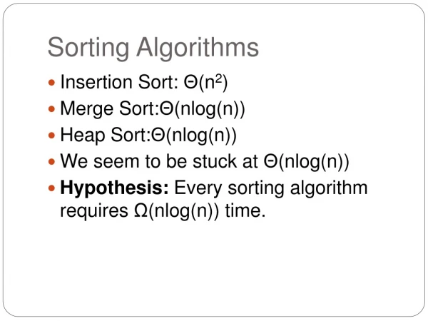
Sorting So Far • Insertion sort: • Easy to code • Fast on small inputs (less than ~50 elements) • Fast on nearly-sorted inputs • O(n2) worst case • O(n2) average (equally-likely inputs) case
Sorting So Far • Merge sort: • Divide-and-conquer: • Split array in half • Recursively sort subarrays • Linear-time merge step • O(n lg n) worst case • Doesn’t sort in place
Sorting So Far • Heap sort: • Uses the very useful heap data structure • Complete binary tree • Heap property: parent key > children’s keys • O(n lg n) worst case • Sorts in place • Fair amount of using memory
Sorting So Far • Quick sort: • Divide-and-conquer: • Partition array into two subarrays, recursively sort • All of first subarray < all of second subarray • No merge step needed! • O(n lg n) average case • Fast in practice • O(n2) worst case • worst case on sorted input • randomized quicksort
Sorting in Linear Time • The sorting algorithms we introduced so far determine the sort order based only on comparisons between the input elements( comparison sorts). • We will examine three sorting algorithms counting sort, radix sort, and bucket sort -that run in linear time • These algorithms use operations time. other than comparisons to determine the sorted order.
Sorting In Linear Time • Counting sort • No comparisons between elements! • But…depends on assumption about the numbers being sorted • We assume numbers are in the range 1..k • The algorithm: • Input: A[1..n], where A[j] {1, 2, 3, …, k} • Output: B[1..n], sorted (notice: not sorting in place) • Also: Array C[1..k] for auxiliary storage
Counting sort Counting sort assumes that each of the n input elements is an integer in the range 0 to k, for some integer k. The basic idea of counting sort is to determine, for each input element x, the number of elements less than x. This information can be used to place element x directly into its position in the output array. In the code for counting sort, we assume that the input is an array [1 … n], and thus length [A]= n. We require two other arrays: the array B[1 …n] holds the sorted output, and the array C[0 … k] provides temporary working storage.
Counting Sort 1 Counting-Sort(A, B, k) 2 for i=1 to k 3 C[i]= 0; 4 for j=1 to n 5 C[A[j]] += 1; 6 for i=2 to k 7 C[i] = C[i] + C[i-1]; 8 for j=n downto 1 9 B[C[A[j]]] = A[j]; 10 C[A[j]] - = 1;
Takes time O(k) Takes time O(n) Counting Sort 1 Counting-Sort(A, B, k) 2 for i=1 to k 3 C[i]= 0; 4 for j=1 to n 5 C[A[j]] += 1; 6 for i=2 to k 7 C[i] = C[i] + C[i-1]; 8 for j=n downto 1 9 B[C[A[j]]] = A[j]; 10 C[A[j]] -= 1; What will be the running time?
Counting Sort • Total time: O(n + k) • Usually, k = O(n) • Thus counting sort runs in O(n) time An important property of counting sort is that is stable : numbers with the same value appear in the output array in the same order as they do in the input array.
Counting Sort • Why don’t we always use counting sort? • Because it depends on range kof elements • Could we use counting sort to sort 32 bit integers? Why or why not? • Answer: no, k too large (232 = 4,294,967,296)
Counting Sort Non-comparison sort. Precondition: n numbers in the range 1…..k. Key ideas: For each x count the number C(x) of elements ≤ x Insert x at output position C(x) and decrement C(x).
1 2 3 4 5 6 7 2 2 2 2 1 0 2 Auxiliary storage C[1..k] 1 2 3 4 5 6 7 2 4 6 8 9 9 11 C An Example 1 2 3 4 5 6 7 8 9 10 11 Input 7 1 3 1 2 4 5 7 2 4 3 A[1..n] k for j=1 to n C[A[j]] + = 1; two 1’s in A for i = 2 to 7 do C[i] = C[i] + C[i–1] 6 elements ≤ 3
1 2 3 4 5 6 7 8 9 10 11 Output B[1..n] 1 2 3 4 5 6 7 C 2 4 6 8 9 9 11 1 2 3 4 5 6 7 2 4 5 8 9 9 11 C 1 2 3 4 5 6 7 8 9 10 11 Input 7 1 3 1 2 4 5 7 2 4 3 A[1..n] 3 B[6] =B[C[3]] =B[C[A[11]]] =A[11] = 3 C[A[11]] =C[A[11]] – 1
1 2 3 4 5 6 7 2 4 5 7 9 9 11 C 1 2 3 4 5 6 7 8 9 10 11 Input 7 1 3 1 2 4 5 7 2 4 3 1 2 3 4 5 6 7 8 9 10 11 3 4 B B[C[A[10]]] =A[10] = 4 1 2 3 4 5 6 7 C 2 4 5 8 9 9 11 C[A[10]] =C[A[10]]– 1
1 2 3 4 5 6 7 8 9 10 11 Input 7 1 3 1 2 4 5 7 2 4 3 1 2 3 4 5 6 7 8 9 10 11 2 3 4 4 5 7 B B[C[A[6]]] =A[6] = 4 1 2 3 4 5 6 7 C 2 3 5 7 8 9 10 C[A[6]] =C[A[6]] – 1 1 2 3 4 5 6 7 2 3 5 6 8 9 10 C
Pass 1: Radix Sort Sort a set of numbers in multiple passes, starting from the rightmostdigit, then the 10’s digit, then the 100’s digit, etc. Example: sort 23, 45, 7, 56, 20, 19, 88, 77, 61, 13, 52, 39, 80, 2, 99 99 77 80 2 13 39 7 88 20 61 52 23 45 56 19 Pass 2: 88 7 23 56 19 61 77 80 99 20 52 2 13 39 45
Analysis of Radix Sort Correctness follows by induction on the number of passes. Sort n d-digit numbers. Let k be the range of each digit. Each pass takes time (n+k). // use counting sort There are d passes in total. The running time for radix sort is(dn+dk). Linear running time when d is a constant and k = O(n).
Radix Sort • Key idea: sort the least significant digit first RadixSort(A, d) for i=1 to d StableSort(A) on digit i
Radix Sort • In general, radix sort based on counting sort is • Fast • Asymptotically fast (i.e., O(n)) • Simple to code • A good choice
Bucket Sort • Assumption: input - nreal numbers from [0, 1) • Basic idea: • Create n linked lists (buckets) to divide interval [0,1) into subintervals of size 1/n • Our code for bucket sort assumes that the input is an n element array A and that each element A[i] in the array satisfies 0 ≤ A[i] < 1. • Add each input element to appropriate bucket and sort buckets with insertion sort • Uniform input distribution O(1) bucket size • Therefore the expected total time is O(n)
Bucket Sort Bucket-Sort(A) n length(A) fori 0 to n do insert A[i] into list B[floor(n*A[i])] // O(n) fori 0 to n –1 do Insertion-Sort(B[i]) // Concatenate lists B[0], B[1], …B[n –1] in order //O(n)
Bucket Sort Taking expectations of both sides: E(T(n))=E(O(n)) + E( )= O(n) + E( ) = O(n) +[ 2- (1/n) ] = O(n)
.12 .17 .21 .23 .26 .39 .68 .72 .78 .94 Bucket Sort Example 0 1 .12 .17 2 .21 .23 .26 3 .39 4 5 6 .68 7 .72 .78 8 9 .94 Bucket i holds values in the half-open interval [i/10, (i + 1)/10).
Bucket sort n +(n+100).0175n + 18n 3.5n 645 35246 2 2 Comparison of Sorting Methods (II) Method Space Average Max n=16 n=10000 Counting sort 2n + 1000 22n + 10010 22n 10362 32010 Radix sort n +(n+200) 32n 32n + 4838 4250 36838
Comparison of Sorting Algorithms Insertion sort: suitable only for small n. Merge sort: guaranteed to be fast even in its worst case; stable. Heapsort: requiring minimum memory and guaranteed to run fast; average and maximum time both roughly twice the average time of quicksort. Quicksort: most useful general-purpose sorting for very little memory requirement and fastest average time. (choose the median of three elements as pivot in practice :-) Counting sort: very useful when the keys have small range; stable; Radix sort: appropriate for keys that are short Bucket sort: assuming keys to have uniform distribution.