Download
1 / 46
480 likes | 520 Views
Learn about parallel and distributed algorithms, including the Divide-and-Conquer paradigm and parallel merge-sort. Explore sorting algorithms like Merge-Sort and Quick-Sort, along with performance analysis and time complexity notations.

E N D
Lecture 7 :Parallel Algorithms(focus on sorting algorithms) Courtesy : SUNY-Stony Brook Prof. Chowdhury’s course note slides are used in this lecture note
Parallel/Distributed Algorithms • Parallel program(algorithm) • A program (algorithm) is divided into multiple processes(threads) which are run on multiple processors • The processors normally are in one machine execute one program at a time have high speed communications between them • Distributed program(algorithm) • A program (algorithm) is divided into multiple processes which are run on multiple distinct machines • The multiple machines are usual connected by network. Machines used typically are workstations running multiple programs.
Divide-and-Conquer • Divide • divide the original problem into smaller subproblems that are easier are to solve • Conquer • solve the smaller subproblems (perhaps recursively) • Merge • combine the solutions to the smaller subproblems to obtain a solution for the original problem Can be extended to parallel algorithm
Divide-and-Conquer • The divide-and-conquer paradigm improves program modularity, and often leads to simple and efficient algorithms • Since the subproblems created in the divide step are often independent, they can be solved in parallel • If the subproblems are solved recursively, each recursive divide step generates even more independent subproblems to be solved in parallel • In order to obtain a highly parallel algorithm it is often necessary to parallelize the divide and merge steps, too
Example of Parallel Program(divide-and-conquer approach) • spawn • Subroutine can execute at the same time as its parent • sync • Wait until all children are done • A procedure cannot safely use the return values of the children it has spawned until it executes a sync statement. Fibonacci(n) 1: if n < 2 2: return n 3: x = spawn Fibonacci(n-1) 4: y = spawn Fibonacci(n-2) 5: sync 6: return x + y
Performance Measure • Tp • running time of an algorithm on p processors • T1 • running time of algorithm on 1 processor • T∞ • the longest time to execute the algorithm on infinite number of processors.
Performance Measure • Lower bounds on Tp • Tp >= T1 / p • Tp >= T∞ • P processors cannot do more than infinite number of processors • Speedup • T1 / Tp : speedup on p processors • Parallelism • T1 / T∞ • Max possible parallel speedup
Related Sorting Algorithms • Sorting Algorithms • Sort an array A[1,…,n] of n keys (using p<=n processors) • Examples of divide-and-conquer methods • Merge-sort • Quick-sort
Merge-Sort • Basic Plan • Divide array into two halves • Recursively sort each half • Merge two halves to make sorted whole
Time Complexity Notation • Asymptotic Notation (점근적 표기법) • A way to describe the behavior of functions in the limit • (어떤 함수의 인수값이 무한히 커질때, 그 함수의 증가율을 더 간단한 함수를 이용해 나타내는 것)
Time Complexity Notation • O notation – upper bound • O(g(n)) = { h(n): ∃ positive constants c, n0 such that 0 ≤ h(n) ≤ cg(n), ∀ n ≥ n0} • Ω notation – lower bound • Ω(g(n)) = {h(n): ∃ positive constants c > 0, n0 such that 0 ≤ cg(n) ≤ h(n), ∀ n ≥ n0} • Θ notation – tight bound • Θ(g(n)) = {h(n): ∃ positive constants c1, c2, n0 such that 0 ≤ c1g(n) ≤ h(n) ≤ c2g(n), ∀ n ≥ n0}
Performance Analysis Too small! Need to parallelize Merge step
(Sequential) Quick-Sort algorithm • a recursive procedure • Select one of the numbers as pivot • Divide the list into two sublists: a “low list” containing numbers smaller than the pivot, and a “high list” containing numbers larger than the pivot • The low list and high list recursively repeat the procedure to sort themselves • The final sorted result is the concatenation of the sorted low list, the pivot, and the sorted high list
(Sequential) Quick-Sort algorithm • Given a list of numbers: {79, 17, 14, 65, 89, 4, 95, 22, 63, 11} • The first number, 79, is chosen as pivot • Low list contains {17, 14, 65, 4, 22, 63, 11} • High list contains {89, 95} • For sublist {17, 14, 65, 4, 22, 63, 11}, choose 17 as pivot • Low list contains {14, 4, 11} • High list contains {64, 22, 63} • . . . • {4, 11, 14, 17, 22, 63, 65} is the sorted result of sublist • {17, 14, 65, 4, 22, 63, 11} • For sublist {89, 95} choose 89 as pivot • Low list is empty (no need for further recursions) • High list contains {95} (no need for further recursions) • {89, 95} is the sorted result of sublist {89, 95} • Final sorted result: {4, 11, 14, 17, 22, 63, 65, 79, 89, 95}
Randomized quick-sort Par-Randomized-QuickSort ( A[ q : r ] ) 1. n <- r ― q + 1 2. if n <= 30 then 3. sort A[ q : r ] using any sorting algorithm 4. else 5. select a random element x from A[ q : r ] 6. k <- Par-Partition ( A[ q : r ], x ) 7. spawnPar-Randomized-QuickSort ( A[ q : k ― 1 ] ) 8. Par-Randomized-QuickSort ( A[ k + 1 : r ] ) 9. sync • Worst-Case Time Complexity of Quick-Sort : O(N^2) • Average Time Complexity of Sequential Randomized Quick-Sort : O(NlogN) • (recursion depth of line 7-8 is roughly O(logN). Line 5 takes O(N))
Parallel partition • Recursive divide-and-conquer