Download
1 / 25
250 likes | 457 Views
Surface Energy and Surface Stress in Phase-Field Models of Elasticity. J. Slutsker , G. McFadden, J. Warren, W. Boettinger, (NIST). K. Thornton , A. Roytburd, P. Voorhees, (U Mich, U Md, NWU). Surface excess quantities and phase-field models

E N D
Surface Energy and Surface Stress in Phase-Field Models of Elasticity J. Slutsker, G. McFadden, J. Warren, W. Boettinger, (NIST) K. Thornton, A. Roytburd, P. Voorhees, (U Mich, U Md, NWU) • Surface excess quantities and phase-field models • 1-D Elastic equilibrium – axial stress & biaxial strain • 3-D Equilibrium of two-phase spherical systems Goal: illuminate phase-field description of surface energy and surface strain by simple examples
Kramer’s Potential (fluid system) (surface energy)
1-D Elastic System (single component) z “Liquid” Solid
Planar Geometry z • Solid and “liquid” separated by an interface • Planar geometry • No dynamics • Applied uniaxial stress or biaxial strain • 1D problem t0 Liquid eS Solid • Examine • Equilibrium temperature (T0) • Surface energy and surface stress (Gibbs adsorption) • Analytical results and numerical results are compared
Here is the analytical results for the melting temperature. Using the first integral of the system, we obtain the constant quantity that gives equilibrium. Here, f is the free energy including the temperature effect, fel is the elastic energy density, this is the gradient energy, and the last term is the work term due to applied stress, where tau0 is the applied stress, U’ is the strain ezz. Using analytic solution for the elastic equilibrium, we obtain this expression for the melting temperature shift due to the presence of applied stress or applied strain. Note that the shift depends only on the jump of the quantities, and does not depend on the interfacial thickness. Analytical Results: Melting Temperature • First integral • We thus obtain, • where [[ ]] denotes the jump across the interface
For numerical simulation, we take a physical parameter for Aluminum eutectic (or an estimate for it. The equations are non-dimensionalized using the latent heat per unit volume and the system size. We now focus on the case with applied stress only, that is tau0 is non zero, and msifit and applied strain is zero. Then the expression for the melting temperautre change becomes this. The change is proportional to the applied stress^2. Numerical Simulation: Melting Temperature • “Physical” parameters for Aluminum eutectic is used • Variables are non-dimensionalized using the latent heat per unit volume and the system length • Here, we focus on applied stress with no misfit:
Simulation and analytics agree • Indeed the simulation results agree with the analytical results.
Analytical Results: Surface Energy • Surface energy is associated with the surface excess of thermodynamic potential [Johnson (2000)] • “Gibbs adsorption equation” can be derived [Cahn (1979)]:
Numerical and analytical results agree • Here, I plot dgama dtau0 agaist tau0. The numerical solution agrees with the analytical solution for dgamma dtau0.
Elastic Equilibrium of a Spherical Inclusion L S T uS=0 Bulk modulus, KL=KS=K Shear modulus, m=0 in “liquid” VS<VL Self-strain: e0djk in liquid 0 in solid (1) (2) R1 R Df=fS-fL= LV (T-T0)/T0 Compare phase-field & sharp interface results for Claussius-Clapyron/Gibbs-Thomson effects [numerics & asymptotics] [Johnson (2001)]
Solid Inclusion S L
Liquid Inclusion L S
Phase-Field Calculations Liquid fraction S L T/T0 Liquid-Solid volume mismatch produces stress and alters equilibrium temperature (Claussius-Clapyron)
Phase Field vs Sharp Interface (no surface energy) Liquid fraction
Phase Field vs Sharp Interface (surface energy fit) T/T0 Liquid fraction
Conclusions • Phase-field models provide natural surface excess quantities • Surface stress is included – but sensitive to interpolation through the interface • Surface energy and Clausius-Clapyron effects included Future Work • More detailed numerical evaluation of surface stress in 3-D • Derive formal sharp-interface limit of phase-field model