Frequency (Hz)

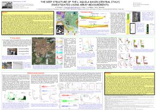
1. North A-A’ B-B’ S2 S3 S8 S8 Italy L’Aquila EW velocity (m/s) NS UP 1 hour 0.5 s 1 s THE DEEP STRUCTURE OF THE L'AQUILA BASIN (CENTRAL ITALY) INVESTIGATED USING ARRAY MEASUREMENTS ESG4 Conference @ UCSB 4th IASPEI / IAEE International Symposium: Effects of Surface Geology on Seismic Motion. University of California, Santa Barbara, August 23-26, 2011 Poster Session 1:  Recent Significant Earthquakes  Paper No. 1.8 velocity (m/s) G. Di Giulio 1,2 (giuseppe.digiulio@ingv.it), F. Cara 1,2, G. Milana 1, and I. Gaudiosi 2 (1) Istituto Nazionale di Geofisica e Vulcanologia, Rome, Italy, (2) DISAT, Dipartimento di Ingegneria delle Strutture, delle Acque e del Terreno, Università degli Studi dell’Aquila, L’Aquila, Italy SMP AN PZZ 1 Geological setting Abstract We present velocity profiles obtained through surface-wave methods in the historical city of L’Aquila (Italy). The city suffered severe damage (VIII-IX EMS intensity) during the April 6th 2009 Mw 6.3 earthquake (Tertulliani et al., 2011). The area is characterized by the deep (up to 300-400 meters) basin of the Aterno river valley filled by lacustrine sediments over limestone bedrock. An outcropping quaternary unit basically composed of stiff Breccia conglomerates (Br) is over-imposed to ancient lacustrine sediments (L) in downtown L’Aquila, with a possible velocity inversion at a depth ranging from few tens up to one hundred meters. Five 2-D arrays of seismic stations and one 1-D array of vertical geophones were deployed in the city center. The 2-D arrays recorded ambient noise, whereas the 1-D array recorded signals produced by an active source. Surface-wave dispersion and spatial autocorrelation curves, calculated using array methods, were inverted through a improved neighborhood algorithm (Wathelet, 2008) jointly with the microtremor H/V ellipticity. Shear-wave velocity (Vs) profiles representative of the average behavior for the southern and northern downtown have been obtained. The resulting Vs profiles allowed us to compare the 1-D transfer functions to aftershock spectral ratio results. We then applied a convolution approach composed of two steps for evaluating synthetic time-histories at a strong-motion site where the near-surface geology is well known. The Vs profile obtained by surface-wave analysis was first used for deconvolving at the bedrock level the mainshock time-history recorded at one strong-motion station (AQK) deployed in the southern downtown. We then convolved the bedrock-input-motion with an available soil profile through an equivalent-linear approach (Bardet et al., 2000); we estimated the surface ground-motion at the strong-motion site (AQV) which recorded the maximum PGA (~0.66 g) during the L’Aquila mainshock. S2 Filling and residual soils Fig. 2a – Stratigraphic column derived from a deep borehole performed in the framework of the microzoning activities (S2 survey situated in “Piazza Duomo”; http://www.cerfis.it). The borehole shows the transition between Br and L at a deep around 100 m, and a thickness of more than 200 m of L (Amoroso et al., 2010). L’Aquila terrace is composed (from top to bottom) of alluvial Quaternary breccias (Br), Lower-Pleistocene lacustrine sediments (L; silty and sandy layers) and limestone (Fig. 1). Stiff breccias (Br) are outcropping in the north of the city and along the terrace flanks, thin uppermost layers of colluvial soil (“limi rossi”, Lr) are outcropping mostly in the south downtown, L deposits outcrop at the base of the terrace within the Aterno river valley. The contact between Br and L is responsible of a velocity inversion (Figures 2-a and 2-b). Vs is quite high for Br reaching values around 1000 m/s, whereas the Vs of superficial Lr deposits drops down to 300-400 m/s. The mean value of Vs for L is around 600 m/s (Fig. 2b). AS 8 m AL 1 Km Downtown L’Aquila Section A-A’ 1D MASW Breccias formation (Br) Frequency (Hz) S2 S8 B-B’ Breccia (Br) Lacustrine deposits (L) 80/100 m Lacustrine sediments (L) Limestone 300 m Fig. 2b – Left) The S3 cross-hole profile was performed at the base of L’Aquila terrace (L unit; (Cardarelli and Cercato, 2010). Right) The velocity inversion was found by the S8 downhole survey at a depth of about 40 m (i.e. transition from Br to L). S3 Downtown L’Aquila 4 m Limi Rossi (Lr) Section B-B’ S2 S3 Vs A-A’ Lacustrine sediments (L) Breccias (Br1) Vs Vp Fig. 1- Left) Geological setting of the L’Aquila area; the downtown is bounded by the dashed black curve. The L’Aquila terrace slopes down in the southwest direction, raising about 50 meters above the Aterno river bed. S2, S3 and S8 indicate the position of borehole and downhole surveys shown in Figure 2 (http://www.cerfis.it). Right) Geological sections after the Microzoning activity of the Italian Civil Defense Department (DPC; http://www.protezionecivile.it/jcms/it/microzonazione_aquilano.wp). Alluvial deposits Brecce di S. Giuliano Limi Rossi Brecce dell’Aquila Lacustrine sediments (L) Lacustrine deposits (lower Pleistocene) Limestone 80 m 2 Array analysis The surface-wave dispersion curves (SWDCs) of the two 2D arrays arranged in south downtown (AS and AL) and of the 1D MASW array show very consistent trends in the frequency range 0.8 - 40 Hz (Fig. 5). Therefore, we combine the SWDCs of AS, AL and 1D MASW array considering the merged curve as representative of the southern part of the city. The shape of the merged curve suggests an effect related to a velocity reversal of the subsoil profile (Fig. 5), interpreted as the contact between Br and the L (see Figures 1 and 2). In the northern downtown, the SWDCs provided by the three arrays (AN, SMP and PZZ) show persistently larger apparent phase-velocities than those measured in the southern downtown (Fig. 5). In contrast to what observed in the southern part, the SWDCs of AN, SMP and PZZ arrays are not overlapping. The very high apparent phase-velocities measured by PZZ and SMP arrays cannot be merged with the velocities of the largest AN array (Fig. 5). This suggests that local high-velocity heterogeneities of the geotechnical structure could play an important role in the northern downtown (Fig. 6). The velocities profiles assessed by a joint inversion (dispersion, spatial autocorrelation curves and microtremor HVNSR ellipticity) through an improvedneighborhood algorithm (Wathelet, 2008) are reported in Figures 7 and 8. The H/V noise spectral ratios (HVNSR) are fairly in agreement for each 2D array, showing a fundamental resonance frequency (f0) varying between 0.5 and 0.6 Hz (Fig. 3). The HVNSR curves show the strongest peaks in the southern part of the city (i.e. AS and AL arrays). In the northern part (i.e. AN, PZZ and SMP arrays) the HVNSRs show the lowest values of f0 (~ 0.5 Hz) and the corresponding H/V amplitude is less strong (Milana et al., 2011). A surface-waves analysis has been applied to vertical signals recorded by 2D and 1D arrays. We applied frequency-wavenumber (F-K; Lacoss et al., 1969; Capon, 1969) and spatial autocorrelation methods (SPAC; Aki, 1957; Bettig et al., 2001) through the geopsy analysis tool (www.geopsy.org). Five 2D arrays of seismic stations (named PZZ, AN, AS, SMP and AL) were installed in downtown in different time-periods. We used array apertures ranging from 100 m up to 1 km with a number of remote stations varying from 12 to 15 for each single array (Figures 3 and 4a). The experiment consisted also of a linear array of vertical 4.5 Hz geophones (Fig. 4b) recording passive as well as active data through a mini-gun for investigating the high-frequency range (> 10 Hz). 1000 m 0 Fig. 7 –Inversion results for the AN array, deployed in the northern downtown. The black curves show the experimental data, and the colored curves the fitting inverted models (the color scale varies with misfit values). The inverted Vp and Vs profiles are shown on the right-hand side panel. Fig. 5 – Surface-wave dispersion curves (SWDCs) derived from F-K analysis. The arrays in the southern part of the city (AS, AL and the 1-D MASW survey) provide SWDCs with consistent apparent phase-velocities in the overlapping frequencies. The SWDCs related to northern arrays (AN, SMP and PZZ) are not overlapping. Breccia (Br) Lacustrine deposits (L) Fig. 4a - The seismic stations within the 2-D arrays were composed of Reftek130 or MarLite digitizers connected to 5sec sensors (Le3d-5s) and recorded hours of ambient seismic noise. The time synchronization for each station was provided by a GPS antenna. The sampling rate was fixed to 250 Hz. The stations position was obtained by differential GPS measurements through a real time kinematic survey using a Leica 1200 GNSS GPS instrument. Limestone 1000 m 0 R1 R0 R2 SMP Fig. 4b – The linear array was composed of 72 vertical 4.5 Hz geophones with a regular spacing of 1 m. We used a minigun as active source performing eight shots at different offsets. PZZ Fig. 3 – Map showing the five 2-D arrays (PZZ, AN, AS, SMP and AL) installed in the city. The linear array of geophones is shown as thick black line (MASW). The triangles show the FAQ2, MARG, AQU and AQK stations. FAQ2 and MARG were used for the computation of classical spectral ratios (HHSR in Fig. 9); AQU and AQK are strong-motion stations that recorded the Mw 6.3 L’Aquila mainshock (PGA ~ 300-350 cm/s2, PGV ~ 35 cm; Çelebi et al., 2010). Fig. 8 –Inversion results for the arrays deployed in the southern downtown (combining AS, AL and the 1D MASW arrays). The black curves show the experimental data, and the colored curves the inverted models (the color scale varies with misfit values). The inverted Vp and Vs profiles are shown on the right-hand side panel. Fig. 6 –The SWDC of the SMP and PZZ arrays can be interpreted assuming a 50 m thick layer of Br (Vs ~ 1000 m/s) over a high-velocity body, and invoking a role of the first higher mode of Rayleigh wave (R1) from 15 to 25 Hz. 3 Bedrock motion evaluation Conclusion We investigated the S-wave velocity structure of L’Aquila city by surface-wave analysis combining several 2-D arrays of seismological sensors with different apertures and 1-D array of geophones. For the southern downtown, a surface-wave dispersion curve (SWDC) was obtained in a large frequency band (0.8-40 Hz) by merging the curves from two 2-D arrays (AS and AL) and the curve provided by the 1-D MASW survey (Fig. 5). The analysis evidenced the role of a velocity inversion (likely affecting both Vp and Vs profiles) related to the contact between stiff Breccia (Br) and underlying ancient lacustrine deposit (L). For the northern downtown, it was not possible to combine the SWDC of the corresponding arrays (AN, SMP and PZZ) indicating a more complex situation. We suppose that the presence of very high-velocity body could mask the effect of a velocity inversion related to deepest unresolved L layer. This observation seems confirmed by a reflection seismic profile performed in the area and still under elaboration (Di Fiore, personal communication) We then assessed the bedrock-input-motion by deconvolving the Mw 6.3 mainshock recorded at the AQK strong-motion site using the inverted Vs model obtained through the joint inversion. The bedrock-input-motion was convolved with the near-surface properties of the strong-motion site (AQV) that recorded the maximum PGA during the L’Aquila Mw 6.3 mainshock. Although near-source and 2-D/3-D effects were not considered by our analysis, a generally good agreement was observed between the ground motion recorded at AQV and the solution provided by the equivalent-linear approach including soil nonlinearity. This suggests the possibility of using the obtained bedrock-input-motion in analysis aimed at evaluating the seismic response for the area. The bedrock-input-motion obtained in Fig. 10 can be used for determining surface strong-motion synthetics at sites with a good knowledge of the near-surface geology. We applied this method to the strong-motion site AQV (Fig. 11) which recorded the maximum PGA during the Mw 6.3 L’aquila mainshock (PGA of 644 cm/s2; Çelebi et al., 2010). AQV is situated 5 km NW from downtown L’Aquila in the middle Aterno river valley and an accurate site characterization was performed during the microzoning activity (see http://itaca.mi.ingv.it/ItacaNet/). Because nonlinear effects can occur at AQV, the convolution through the equivalent-linear approach (Bardet et al., 2000) was performed accounting the soil nonlinearity as well as adopting a constant shear modulus with no damping variation. In the former case, we allowed variation of shear modulus and damping ratio with shear strain (Figures 11 and 12). The Vs model obtained by surface-wave analysis for the southern downtown (Fig. 8) has been used to deconvolve at the bedrock level the L’Aquila Mw 6.3 mainshock recorded at the AQK strong-motion site (Fig. 3). The deconvolution was obtained using an equivalent-linear approach through the EERA software (Bardet et al., 2000). Due to the soil material properties we did not include soil nonlinearity for both Br and L deposits. The deconvolution at the bedrock level of the Mw 6.3 earthquake recorded at AQK produced a reduction of PGA from 0.33 to 0.17 g (Fig. 10). Because the arrays have a large spatial extension, the Vs profiles of Figures 7 and 8 are representative of average properties of the respective areas. In both areas, the joint inversion assuming the fundamental mode of Rayleigh waves resolves the velocity inversion related to the contact between Br and L deposits, with the largest thickness found for northern downtown. The best-fitting inverted models (Figures 7 and 8) have been used to compute the 1-D theoretical transfer function for vertically incident SH plane-waves. The 1-D SH transfer functions are compared to the experimental amplification functions derived from aftershock data analysis (Fig. 9). We considered the classical spectral ratios using a rock reference site (HHSR) for two seismic stations (FAQ2 and MARG) situated in the southern and northern downtown, respectively (see Fig. 3). The agreement is quite good for both stations considering all the uncertainties at the base of 1-D modeling. Br L Fig. 11 – AQV site: soil column, Vs profile from the cross-hole data and H/V noise curve. We assumed the material properties suggested by Vucetic and Dobry (1991) with plasticity index 50% for clay; the curves proposed by Seed et al. (1986) for sand; we adopted an average curve deduced by available literature data for gravel (Tito Sanò, personal communication). References:Aki, K. [1957], “Space and time spectra of stationary stochastic waves, with special reference to microtremors’’, Bull. Earthq. Res. Inst., Vol. 35, pp. 415–456. Amoroso, S., F. Del Monaco, F. Di Eusebio, et al. [2010], “Campagna di indagini geologiche, geotecniche e geofisiche per lo studio della risposta sismica locale della città dell'Aquila: la stratigrafia dei sondaggi (Giugno - Agosto 2010)’’, CERFIS Report, pp. 1-51, http://www.cerfis.it/it/attivita/microzonazione.html, in Italian. Bardet, J. P.,K. Ichii, and C. H. Lin [2000], ‘’EERA, a computer program for equivalent-linear earthquake site response analyses of layered soil deposits, University of Southern California, Department of Civil Engineering’’, http://gees.usc.edu/GEES/. Bertrand, E., A. M. Duval, J. Régnier, et al. [2011], “Site effects of the Roio basin, L’Aquila”, Bull. Earthquake Eng., doi:10.1007/s10518-011-9254-6. Bettig, B.,P. Y. Bard, F. Scherbaum, J. Riepl, F. Cotton, C. Cornou, and D. Hatzfeld [2001], “Analysis of dense array noise measurements using the modified spatial autocorrelation method (SPAC). Application to the Grenoble area’’, Boll. Geof. Teor. Appl., Vol. 42, No. 3-4, pp. 281-304. Capon, J. [1969], “High-resolution frequency-wavenumber spectrum analysis’’, Proc. of the IEEE, Vol. 57, No. 8, pp. 1408–1418. Cardarelli, E., and M. Cercato [2010], “Relazione sulla campagna d'indagine geofisica per lo studio della risposta sismica locale della città dell'Aquila, Prova Crosshole Sondaggi S3-S4’’, DICEA Report, pp. 1-13, http://www.cerfis.it/it/attivita/microzonazione.html, in Italian. Çelebi, M., P. Bazzurro, L. Chiaraluce, et al. [2010], “Recorded Motions of the 6 April 2009 Mw 6.3 L’Aquila, Italy, Earthquake and Implications for Building Structural Damage: Overview’’, Earthquake Spectra, Vol. 26, No. 3, pp. 651-684, doi:10.1193/1.3450317. Lacoss, R. T.,E. J. Kelly, and M. N. Toksoz [1969], “Estimation of seismic noise structure using arrays’’, Geophysics, Vol. 34, pp. 21-38. Milana, G., R. M. Azzara, E. Bertrand, et al. [2011], “The contribution of seismic data in microzonation studies for downtown L’Aquila’’, Bull. Earthquake Eng., Vol. 9, No. 3, pp. 741-759, doi: 10.1007/s10518-011-9246-6. Seed, H. B., R. T. Wong, I. M. Idriss, and K.Tokimatsu [1986], “Moduli and damping factors for dynamic analyses of cohesionless soils’’, J. Geotech. Eng. Div., ASCE, Vol. 112 (GT11), pp. 1016-1032. Tertulliani, A., L. Arcoraci, M. Berardi, et al. [2011],‘ ’An application of EMS98 in a medium-sized city: The case of L’Aquila (Central Italy) after the April 6, 2009 Mw 6.3 earthquake’’, Bull. Earthquake Eng., Vol. 9, pp. 67–80, doi 10.1007/s10518-010-9188-4. Vucetic, M. and R. Dobry [1991], “Effects of the soil plasticity on ciclyc response’’, J. Geotech. Eng. Div., ASCE, Vol. 117, No.1, pp. 898-907. Wathelet, M. [2008], “An improved neighborhood algorithm: parameter conditions and dynamic scaling’’, Geophys. Res. Lett., Vol. 35, L09301, doi:10.1029/2008GL033256. Fig. 9 – Comparison at FAQ2 and MARG sites between the 1-D SH response (black curve) and the HHSR results (green curves; geometrical mean  1 standard deviation). The SH response was computed from the inverted Vs models of Figures 7 and 8. Q values are set equal to the velocities values divided by 10. The HHSRs were computed on ~ 120 local earthquakes collected during the L’Aquila seismic sequence (Milana et al., 2011); the reference site was on a rock outcrops in proximity of the village “Poggio di Roio’’ 2 km SW from L’Aquila (Bertrand et al., 2011). Fig. 10 – Left panel) Vs inverted model assumed for the southern downtown (see Fig. 8). Right-panel) Comparison between the Mw 6.3 time-history recorded at AQK and the bedrock motion after the deconvolution process. The comparison is also performed in terms of response acceleration spectra and Fourier amplitude spectra. Fig. 12 –Comparison between acceleration time-history recorded at AQV (EW component; panel a) and the synthetic acceleration computed through the convolution of the bedrock-input-motion with the soil column of AQV (Fig. 11). The modeling was performed both with and without soil nonlinearity (panel c and b, respectively). The comparison is also shown in terms of response (panel d) and Fourier amplitude spectra (panel e).