Download
1 / 14
150 likes | 173 Views
Single Scattering. Single scattering is the simplest way to spread out a proton beam. It is relatively immune to beam alignment. On the other hand, it is inefficient and wastes more proton energy (range) than we would like.

E N D
Single Scattering Single scattering is the simplest way to spread out a proton beam. It is relatively immune to beam alignment. On the other hand, it is inefficient and wastes more proton energy (range) than we would like. From a pedagogical point of view, a single scattered beam with no modulation is about the only useful beam line that can be designed by hand or, much more easily, with the aid of LOOKUP. To get our feet wet, we’ll run through such a design even before we’ve gotten into the basic physics of proton stopping and scattering. If there are some obscure steps, they may become clear later. Single scattering is essentially Gaussian, so most calculations can be done analytically. Before setting up and solving a sample single scattering problem, we’ll review properties of 1D and 2D Gaussians that we’ll need in this lecture and later.
Single Scattering Problem throw L Single scattered beam. Protons enter with 160 MeV and are to be spread out with dose uniformity ±2.5% over a radius of 1.5 cm at 1.2 meter throw. What material should we use for the scatterer? how much? what is the energy out? the depth in water? If the incident beam current is 1 nA what is the dose rate at the Bragg peak?
Coordinate system. z is in the beam direction, y is up, and xyz form a right-handed frame: x × y = z and so on. Though angles are shown large for clarity, we always work in the small-angle approximation.
1D (Projected) Gaussian The 1D probability density f(θX) of the projected angle is It is usually more convenient to deal with projections on the measuring plane (MP) so we immediately let x = θx× L (small angle) and write It can be shown that f(x) is normalized to 1 and that the rms value of x is equal to the Gaussian width parameter x0 :
2D (Cylindrical) Gaussian If scattering is isotropic as it is for the materials we shall use, the scattering in y equals that in x. Since the two are independent we can find the 2D probability density by multiplying two 1D densities. Doing this and setting r2 = x2 + y2 , y0 = x0 = r0 we find This f(r) is the fluence per proton at the MP: that function which, multiplied by the total number of protons N, is the fluence. Therefore N/(2πr02) is the fluence on axis. As before However
Cylindrical Gaussians (continued) Many writers (Molière, Preston and Koehler) prefer the form and one must take note of which convention is used when navigating the literature. We will use the r0 (or θ0) form, so that the Gaussian width parameter is the same for 1D and 2D but not equal to rms r (or θ) for 2D. The efficiencyε out to a radius R is the fraction of protons that falls within R : or which limits the efficiency of single scattering systems. For instance, if we want ±2.5% dose uniformity, we use the Gaussian out to its 95% point and the efficiency is 5%.
What r0 (or θ0) Do We Require ? is our first question when designing a single scattering system. Suppose as before we want ±2.5% uniformity out to a given radius r95. That leads to whose solution is with the obvious changes if a different dose uniformity is desired.
Single Scattering Problem throw L Single scattered beam. Protons enter with 160 MeV and are to be spread out with dose uniformity ±2.5% over a radius of 1.5 cm at 1.2 meter throw. How much lead do we need? what is the energy out? the depth in water? If the incident beam current is 1 nA what is the dose rate at the Bragg peak?
Single Scattering Solution First, find the required scattering angle. From an earlier slide Now for the hard part: how much lead is required to scatter 160 MeV protons by 0.0390 radians? In an upcoming lecture we will learn Highland’s formula: where LR is the radiation length of the material ( 6.370 g/cm2 for lead) and pv is a kinematic factor we found in an earlier lecture which equals 296.7 MeV at T = 160 MeV. To find L we just have to use trial and error. For instance, assuming L = 1 g/cm2 gives θ0 = 0.0171 radians. Eventually we find that L = 4 g/cm2 gives 0.0368 rad. Even this isn’t strictly correct because the proton loses energy and we should, at each trial, compute the energy loss and use (p1v1p2v2)½ instead of pv.
Comment: Forward and Inverse Problems If we have a formula like and we wish to find θ0 given some material, whose L and LR we know, and some proton energy, it’s no big deal. Use our kinematic relation for pv (assuming the scatterer is not too thick) and plug in the numbers. This is a forward problem. If, however, we need to find the L of a given material that will yield some desired value of θ0, call it C, that’s the inverse problem and it’s much harder because there is no way we can solve for L(θ0) analytically. The point of this slide is that, in the computer age, the inverse problem is also trivial because of routines called ‘root finders’. We know θ0(L) and we merely seek that value of L, call it L′, for which θ0(L′) – C = 0. L′ is said to be a root of the function θ0(L) – C . Root finders, ubiquitous in our programs, are discussed in Numerical Recipes. They work by trial and error but use various smart ways to choose the next trial. Our favorites are False Position (because of the name) and Bisection (bulletproof). Any root finder needs to be told a bracket, that is, the lowest and highest possible value of the solution. That can sometimes be a problem.
Method of False Position ( Regula Falsa ) y = c y = F(x) Find x such that F(x) – c = 0 . In this method (Vaishali Ganit, ca. 3rd century BC) a line is drawn between the last two points to bracket the root, and its intersection with y =c is used for the next bracket. The method is robust --- the root always stays bracketed --- and reasonably fast. We usually use it or the even more robust method of bisection.
Enter LOOKUP LOOKUP is a proton ‘desk calculator’ which makes it easy to solve any proton problem if it can be done by hand at all. (Many beam line designs can’t be done by hand even with this program.) (demonstrate LOOKUP task SINGLE/2) Using LOOKUP we quickly find that the required thickness of lead is 4.181 g/cm2 or 0.368 cm and that the outgoing energy is 148.8 MeV. Ignoring air for the moment, the range of a proton of that energy is 15.55 cm. That is the depth, not of the Bragg peak, but of its distal 80% point d80 . The mass stopping power of 148.8 MeV protons in water is 5.476 MeV/(g/cm2). We can estimate the dose rate at the entrance to the water tank using either the central fluence method or our general formula for dose rate
Single Scattering (continued) The two answers are in fact consistent, since the second formula computes the average dose rate over the design area, which is indeed about 2.5% lower than the central value computed by the first formula. We have, however, made one mistake. We computed the lead thickness taking the design radius at the throw, which is the distance to the Bragg peak, not the tank entrance. The equivalent radius at the tank entrance, 15.5 cm upstream, is a bit smaller and so is the area. Therefore the dose rate is higher (same number of protons through a smaller area → larger fluence). Rather than re-do everything we can just multiply by the ratio of areas, which equals the ratio of distances squared: (120/105)2 = 1.31 . Note this so-called 1/r2 effect is not negligible: entrance dose rate is 30% higher than we said. We’ll have to keep track of it in beam line design, especially for short throw systems. Finally, the dose at the Bragg peak. Our original calculation is correct here insofar as 1/r2 is concerned, but we need to use S/ρ at the Bragg peak, not at 148 MeV. We don’t know S/ρ at the Bragg peak; we don’t even know the proton energy! We do know, though, that the peak/entrance ratio of a measured Bragg peak is always about 3.5 (our fBP) so we can just multiply by that to get 0.135 Gy/sec or 8 Gy/minute.
Summary We have reviewed 1D and 2D Gaussians, noting the √2 difference between two possible definitions of the 2D width parameter (σr = √2 r0). The result means that the efficiency of a single scattering system designed for (say) ±5% dose uniformity will be only 10%. That, and the large energy loss, led to the development of double scattering (ε = 45%) to treat large fields. However, single scattering is useful for small fields and (as we’ll see later) offers by far the smallest lateral penumbra. The parameters of our example were fairly typical of the eye treatment beam line at HCL. With this small area, the dose rate at the Bragg peak is substantial (about 8 Gy/min) even for a beam current as low as 1 nA. An actual eye line at 160 MeV would use a plastic scatterer to intentionally reduce the proton range to ≈4 cm, and would have a selection of range modulators to accommodate lesions of varying extent in depth. Such a system can still be designed from first principles, but not by hand.