Download
1 / 38
390 likes | 600 Views
Interpreting and using heterogeneous choice & generalized ordered logit models. Richard Williams Department of Sociology University of Notre Dame July 2006 http://www.nd.edu/~rwilliam/. The gologit/gologit2 model. The gologit (generalized ordered logit) model can be written as

E N D
Interpreting and using heterogeneous choice & generalized ordered logit models Richard Williams Department of Sociology University of Notre Dame July 2006 http://www.nd.edu/~rwilliam/
The gologit/gologit2 model • The gologit (generalized ordered logit) model can be written as • The unconstrained model gives results that are similar to running a series of logistic regressions, where first it is category 1 versus all others, then categories 1 & 2 versus all others, then 1, 2 & 3 versus all others, etc. • The unconstrained model estimates as many parameters as mlogit does, and tends to yield very similar fits.
The much better known ordered logit (ologit) model is a special case of the gologit model, where the betas are the same for each j (NOTE: ologit actually reports cut points, which equal the negatives of the alphas used here)
The partial proportional odds models is another special case – some but not all betas are the same across values of j. For example, in the following the betas for X1 and X2 are constrained but the betas for X3 are not.
Key advantages of gologit2 • Can estimate models that are less restrictive than ologit (whose assumptions are often violated) • Can estimate models (i.e. partial proportional odds) that are more parsimonious than non-ordinal alternatives, such as mlogit • HOWEVER, there are also several potential concerns users may not be aware of or have not thought about
Concern 1: Unconstrained model does not require ordinality • As Clogg & Shihadeh (1994) point out, the totally unconstrained model arguably isn’t even ordinal • You can rearrange the categories, and fit can be hardly affected • If a totally unconstrained model is the only one that fits, it may make more sense to use mlogit • Gologit is mostly useful when you get a non-trivial # of constraints.
Concern II: Estimated probabilitiescan go negative • Unlike other categorical models, estimated probabilities can be negative. • This was addressed by McCullaph & Nelder, Generalized Linear Models, 2nd edition, 1989, p. 155:“The usefulness of non-parallel regression models is limited to some extent by the fact that the lines must eventually intersect. Negative fitted values are then unavoidable for some values of x, though perhaps not in the observed range. If such intersections occur in a sufficiently remote region of the x-space, this flaw in the model need not be serious.”
Probabilities might go negative in unlikely or impossible X ranges, e.g. when years of education is negative or hourly wages are > $5 million. • But, it could also happen with more plausible sets of values • Multiple tests with 10s of thousands of cases typically resulted in only 0 to 3 negative predicted probabilities. • Seems most problematic with small samples, complicated models, analyses where the data are being spread very thin • they might be troublesome regardless - gologit2 could help expose problems that might otherwise be overlooked • Can also get negative predicted probabilities when measurement of the outcome isn’t actually ordinal
gologit2 now checks to see if any in-sample predicted probabilities are negative. • It is still possible that plausible values not in-sample could produce negative predicted probabilities. • You may want to use some other method if there are a non-trivial number of negative predicted probabilities and you are otherwise confident in your models and data.
Concern III: How do youinterpret the results??? • One rationale for ordinal regression models is that there is an underlying, continuous y* that reflects the dependent variable we are interested in. • y* is unobserved, however. Instead, we observe y, which is basically a collapsed/grouped version of the unobserved y*. • High Income, Moderate Income and Low Income are a collapsed version of a continuous Income variable • Some ranges of attitudes can be collapsed into a 5 category scale ranging from Strongly Disagree to Strongly Agree • As individuals cross thresholds (aka cut-points) on y*, their value on the observed y changes
Question: What does the gologit model mean for the behavior we are modeling? Does it mean the slopes of the latent regression are functions of the left hand side variable, that there is some sort of interaction effect between x and y? i.e. • y* = beta1'x + e if y = 1 • y* = beta2'x + e if y = 2
Further, does the whole idea of an underlying y* go out the window once you allow a single non-proportional effect? If so, how do you interpret the model? • In an ordered logit (ologit) model, you only have one predicted value for y* • But in a gologit model, once you have a single non-parallel effect, you have M-1 linear predictions (similar to mlogit)
Interpretation 1: gologit as non-linear probability model • As Long & Freese (2006, p. 187) point out “The ordinal regression model can also be developed as a nonlinear probability model without appealing to the idea of a latent variable.” • Ergo, the simplest thing may just be to interpret gologit as a non-linear probability model that lets you estimate the determinants & probability of each outcome occurring. Forget about the idea of a y* • Other interpretations, however, can preserve or modify the idea of an underlying y*
Interpretation 2: State-dependent reporting bias - gologit as measurement model • As noted, the idea behind y* is that there is an unobserved continuous variable that gets collapsed into the limited number of categories for the observed variable y. • HOWEVER, respondents have to decide how that collapsing should be done, e.g. they have to decide whether their feelings cross the threshold between “agree” and “strongly agree,” whether their health is “good” or “very good,” etc.
Respondents do NOT necessarily use the same frame of reference when answering, e.g. the elderly may use a different frame of reference than the young do when assessing their health • Other factors can also cause respondents to employ different thresholds when describing things • Some groups may be more modest in describing their wealth, IQ or other characteristics
In these cases the underlying latent variable may be the same for all groups; but the thresholds/cut points used may vary. • Example: an estimated gender effect could reflect differences in measurement across genders rather than a real gender effect on the outcome of interest. • Lindeboom & Doorslaer (2004) note that this has been referred to as state-dependent reporting bias, scale of reference bias, response category cut-point shift, reporting heterogeneity & differential item functioning.
If the difference in thresholds is constant (index shift), proportional odds will still hold • EX: Women’s cutpoints are all a half point higher than the corresponding male cutpoints • ologit could be used in such cases • If the difference is not constant (cut point shift), proportional odds will be violated • EX: Men and women might have the same thresholds at lower levels of pain but have different thresholds for higher levels • A gologit/ partial proportional odds model can capture this
If you are confident that some apparent effects reflect differences in measurement rather than real differences in effects, then • Cutpoints (and their determinants) are substantively interesting, rather than just “nuisance” parameters • The idea of an underlying y* is preserved (Determinants of y* are the same for all, but cutpoints differ across individuals and groups) • You should change the way predicted values are computed, i.e. you should just drop the measurement parameters when computing predictions (I think!)
Key advantage: This could greatly improve cross-group comparisons, getting rid of artifactual differences caused by differences in measurement. • Key Concern: Can you really be sure the coefficients reflect measurement and not real effects, or some combination of real & measurement effects?
Theory may help – if your model strongly claims the effect of gender should be zero, then any observed effect of gender can be attributed to measurement differences. • But regardless of what your theory says, you may at least want to acknowledge the possibility that apparent effects could be “real” or just measurement artifacts.
Interpretation 3: The outcome ismulti-dimensional • A variable that is ordinal in some respects may not be ordinal or else be differently-ordinal in others. E.g. variables could be ordered either by direction (Strongly disagree to Strongly Agree) or intensity (Indifferent to Feel Strongly)
Suppose women tend to take less extreme political positions than men. • Using the first (directional) coding, an ordinal model might not work very well, whereas it could work well with the 2nd (intensity) coding. • But, suppose that for every other independent variable the directional coding works fine in an ordinal model.
Our choices in the past have either been to (a) run ordered logit, with the model really not appropriate for the gender variable, or (b) run multinomial logit, ignoring the parsimony of the ordinal model just because one variable doesn’t work with it. • With gologit models, we have option (c) – constrain the vars where it works to meet the parallel lines assumption, while freeing up other vars (e.g. gender) from that constraint.
This interpretation suggests that there may actually be multiple y*’s that give rise to a single observed y • NOTE: This is very similar to the rationale for the multidimensional stereotype logit model estimated by slogit.
Interpretation 4: The effect of x on y does depend on the value of y • There are actually many situations where the effect of x on y is going to vary across the range of y. • EX: A 1-unit increase in x produces a 5% increase in y • So, if y = $10,000, the increase will be $500. But if y = $100,000, the increase will be $5,000.
If we were using OLS, we might address this issue by transforming y, e.g. takes its log, so that the effect of x was linear and the same across all values of the transformed y. • But with ordinal methods, we can’t easily transform an unobserved latent variable; so with gologit we allow the effect of x to vary across values of y. • This suggests that there is an underlying y*; but because we can’t observe or transform it we have to allow the regression coefficients to vary across values of y instead.
Substantive example: Boes & Winkelman, 2004:Completely missing so far is any evidence whether the magnitude of the income effect depends on a person’s happiness: is it possible that the effect of income on happiness is different in different parts of the outcome distribution? Could it be that “money cannot buy happiness, but buy-off unhappiness” as a proverb says? And if so, how can such distributional effects be quantified?
One last methodological noteon using gologit2 • Despite its name, gologit2 actually supports 5 link functions: logit, probit, log-log, complementary log-log, & Cauchit. Each of these has a somewhat different distribution, differing, for example, in how heavy the tails are and how likely it is you will get extreme values. • Changing the link function may change whether or not a variable meets the parallel lines assumption. • Ergo, before turning to more complicated models and interpretations, you may want to try out different link functions to see if one of them makes it more likely that the parallel lines assumption will hold.
An Alternative to gologit: Heterogeneous Choice (aka Location-Scale) Models • Heterogeneous choice (aka location-scale) models can be generalized for use with either ordinal or binary dependent variables. They can be estimated in Stata by using Williams’ oglm program. (Also see handout p. 3). For a binary outcome,
The logit & ordered logit models assume sigma is the same for all individuals • Allison (1999) argues that sigma often differs across groups (e.g. women have more heterogeneous career patterns). • Unlike OLS, failure to account for this results in biased parameter estimates. • Williams (2006) shows that Allison’s proposed solution for dealing with across-group differences is actually a special case of the heterogeneous choice model, and can be estimated (and improved upon) by using oglm.
Heterogeneous choice models may also provide an attractive alternative to gologit models • Model fits, predicted values and ultimate substantive conclusions are sometimes similar • Heterogeneous choice models are more widely known and may be easier to justify and explain, both methodologically & theoretically
Example: • (Adapted from Long & Freese, 2006 – Data from the 1977 & 1989 General Social Survey) • Respondents are asked to evaluate the following statement: “A working mother can establish just as warm and secure a relationship with her child as a mother who does not work.” • 1 = Strongly Disagree (SD) • 2 = Disagree (D) • 3 = Agree (A) • 4 = Strongly Agree (SA).
Explanatory variables are • yr89 (survey year; 0 = 1977, 1 = 1989) • male (0 = female, 1 = male) • white (0 = nonwhite, 1 = white) • age (measured in years) • ed (years of education) • prst (occupational prestige scale).
See handout pages 2-3 for Stata output • For ologit, chi-square is 301.72 with 6 d.f. Both gologit2 (338.30 with 10 d.f.) and oglm (331.03 with 8 d.f.) fit much better. The BIC test picks oglm as the best-fitting model. • The corresponding predicted probabilities from oglm and gologit all correlate at .99 or higher.
The marginal effects (handout p. 4) show that the heterogeneous choice and gologit models agree (unlike ologit) that the main reason attitudes became more favorable across time was because people shifted from extremely negative positions to more moderate positions • NOTE: In Stata, marginal effects for multiple outcome models are easily estimated and formatted for output by using Williams’s mfx2 program in conjunction with programs like estout and outreg2. • oglm & gologit also agree that it isn’t so much that men were extremely negative in their attitudes; it is more a matter of them being less likely than women to be extremely supportive.
In the oglm printout, the negative coefficients in the variance equation for yr89 and male show that there was less variability in attitudes in 1989 than in 1977, and that men were less variable in their attitudes than women. • This is substantively interesting and relatively easy to explain
Empirically, you’d be hard pressed to choose between oglm and gologit in this case • Theoretical issues or simply ease and clarity of presentation might lead you to prefer oglm • However, see Williams (2006) and Keele & Park (2006) for potential problems and pitfalls with the heterogeneous choice model • Of course, in other cases gologit models may be clearly preferable
For more information, see: http://www.nd.edu/~rwilliam/gologit2 http://www.nd.edu/~rwilliam/oglm/