Download
1 / 30
320 likes | 625 Views
Ordered probit models. Ordered Probit. Many discrete outcomes are to questions that have a natural ordering but no quantitative interpretation: Examples: Self reported health status (excellent, very good, good, fair, poor) Do you agree with the following statement

E N D
Ordered Probit • Many discrete outcomes are to questions that have a natural ordering but no quantitative interpretation: • Examples: • Self reported health status • (excellent, very good, good, fair, poor) • Do you agree with the following statement • Strongly agree, agree, disagree, strongly disagree
Can use the same type of model as in the previous section to analyze these outcomes • Another ‘latent variable’ model • Key to the model: there is a monotonic ordering of the qualitative responses
Self reported health status • Excellent, very good, good, fair, poor • Coded as 1, 2, 3, 4, 5 on National Health Interview Survey • We will code as 5,4,3,2,1 (easier to think of this way) • Asked on every major health survey • Important predictor of health outcomes, e.g. mortality • Key question: what predicts health status?
Important to note – the numbers 1-5 mean nothing in terms of their value, just an ordering to show you the lowest to highest • The example below is easily adapted to include categorical variables with any number of outcomes
Model • yi* = latent index of reported health • The latent index measures your own scale of health. Once yi* crosses a certain value you report poor, then good, then very good, then excellent health
yi = (1,2,3,4,5) for (fair, poor, VG, G, excel) • Interval decision rule • yi=1 if yi* ≤ u1 • yi=2 if u1 < yi* ≤ u2 • yi=3 if u2 < yi* ≤ u3 • yi=4 if u3 < yi* ≤ u4 • yi=5 if yi* > u4
As with logit and probit models, we will assume yi* is a function of observed and unobserved variables • yi* = β0 + x1i β1 + x2i β2 …. xki βk + εi • yi* = xi β + εi
The threshold values (u1, u2, u3, u4) are unknown. We do not know the value of the index necessary to push you from very good to excellent. • In theory, the threshold values are different for everyone • Computer will not only estimate the β’s, but also the thresholds – average across people
As with probit and logit, the model will be determined by the assumed distribution of ε • In practice, most people pick nornal, generating an ‘ordered probit’ (I have no idea why) • We will generate the math for the probit version
Probabilities • Lets do the outliers, Pr(yi=1) and Pr(yi=5) first • Pr(yi=1) • = Pr(yi* ≤ u1) • = Pr(xi β +εi ≤ u1 ) • =Pr(εi ≤ u1 - xi β) • = Φ[u1 - xi β] = 1- Φ[xi β – u1]
Pr(yi=5) • = Pr(yi* > u4) • = Pr(xi β +εi > u4 ) • =Pr(εi > u4 - xi β) • = 1 - Φ[u4 - xi β] = Φ[xi β – u4]
Sample one for y=3 • Pr(yi=3) = Pr(u2 < yi* ≤ u3) = Pr(yi* ≤ u3) – Pr(yi* ≤ u2) = Pr(xi β +εi≤ u3) – Pr(xi β +εi≤ u2) = Pr(εi≤ u3- xi β) - Pr(εi≤ u2 - xi β) = Φ[u3- xi β] - Φ[u2 - xi β] = 1 - Φ[xi β - u3] – 1 + Φ[xi β - u2] = Φ[xi β - u2] - Φ[xi β - u3]
Summary • Pr(yi=1) = 1- Φ[xi β – u1] • Pr(yi=2) = Φ[xi β – u1] - Φ[xi β – u2] • Pr(yi=3) = Φ[xi β – u2] - Φ[xi β – u3] • Pr(yi=4) = Φ[xi β – u3] - Φ[xi β – u4] • Pr(yi=5) = Φ[xi β – u4]
Likelihood function • There are 5 possible choices for each person • Only 1 is observed • L = Σi ln[Pr(yi=k)] for k
Programming example • Cancer control supplement to 1994 National Health Interview Survey • Question: what observed characteristics predict self reported health (1-5 scale) • 1=poor, 5=excellent • Key covariates: income, education, age, current and former smoking status • Programs • sr_health_status.do, .dta, .log
desc; • male byte %9.0g =1 if male • age byte %9.0g age in years • educ byte %9.0g years of education • smoke byte %9.0g current smoker • smoke5 byte %9.0g smoked in past 5 years • black float %9.0g =1 if respondent is black • othrace float %9.0g =1 if other race (white is ref) • sr_health float %9.0g 1-5 self reported health, • 5=excel, 1=poor • famincl float %9.0g log family income
tab sr_health; • 1-5 self | • reported | • health, | • 5=excel, | • 1=poor | Freq. Percent Cum. • ------------+----------------------------------- • 1 | 342 2.65 2.65 • 2 | 991 7.68 10.33 • 3 | 3,068 23.78 34.12 • 4 | 3,855 29.88 64.00 • 5 | 4,644 36.00 100.00 • ------------+----------------------------------- • Total | 12,900 100.00
In STATA • oprobit sr_health male age educ famincl black othrace smoke smoke5;
Ordered probit estimates Number of obs = 12900 • LR chi2(8) = 2379.61 • Prob > chi2 = 0.0000 • Log likelihood = -16401.987 Pseudo R2 = 0.0676 • ------------------------------------------------------------------------------ • sr_health | Coef. Std. Err. z P>|z| [95% Conf. Interval] • -------------+---------------------------------------------------------------- • male | .1281241 .0195747 6.55 0.000 .0897583 .1664899 • age | -.0202308 .0008499 -23.80 0.000 -.0218966 -.018565 • educ | .0827086 .0038547 21.46 0.000 .0751535 .0902637 • famincl | .2398957 .0112206 21.38 0.000 .2179037 .2618878 • black | -.221508 .029528 -7.50 0.000 -.2793818 -.1636341 • othrace | -.2425083 .0480047 -5.05 0.000 -.3365958 -.1484208 • smoke | -.2086096 .0219779 -9.49 0.000 -.2516855 -.1655337 • smoke5 | -.1529619 .0357995 -4.27 0.000 -.2231277 -.0827961 • -------------+---------------------------------------------------------------- • _cut1 | .4858634 .113179 (Ancillary parameters) • _cut2 | 1.269036 .11282 • _cut3 | 2.247251 .1138171 • _cut4 | 3.094606 .1145781 • ------------------------------------------------------------------------------
Interpret coefficients • Marginal effects/changes in probabilities are now a function of 2 things • Point of expansion (x’s) • Frame of reference for outcome (y) • STATA • Picks mean values for x’s • You pick the value of y
Continuous x’s • Consider y=5 • d Pr(yi=5)/dxi = d Φ[xi β – u4]/dxi = βφ[xi β – u4] • Consider y=3 • d Pr(yi=3)/dxi = βφ[xi β – u3] - βφ[xi β – u4]
Discrete X’s • xiβ = β0 + x1i β1 + x2i β2 …. xki βk • X2i is yes or no (1 or 0) • ΔPr(yi=5) = • Φ[β0 + x1i β1 + β2 + x3i β3 +.. xki βk] - Φ[β0 + x1i β1 + x3i β3 …. xki βk] • Change in the probabilities when x2i=1 and x2i=0
Ask for marginal effects • mfx compute, predict(outcome(5));
mfx compute, predict(outcome(5)); • Marginal effects after oprobit • y = Pr(sr_health==5) (predict, outcome(5)) • = .34103717 • ------------------------------------------------------------------------------ • variable | dy/dx Std. Err. z P>|z| [ 95% C.I. ] X • ---------+-------------------------------------------------------------------- • male*| .0471251 .00722 6.53 0.000 .03298 .06127 .438062 • age | -.0074214 .00031 -23.77 0.000 -.008033 -.00681 39.8412 • educ | .0303405 .00142 21.42 0.000 .027565 .033116 13.2402 • famincl | .0880025 .00412 21.37 0.000 .07993 .096075 10.2131 • black*| -.0781411 .00996 -7.84 0.000 -.097665 -.058617 .124264 • othrace*| -.0843227 .01567 -5.38 0.000 -.115043 -.053602 .04124 • smoke*| -.0749785 .00773 -9.71 0.000 -.09012 -.059837 .289147 • smoke5*| -.0545062 .01235 -4.41 0.000 -.078719 -.030294 .081395 • ------------------------------------------------------------------------------ • (*) dy/dx is for discrete change of dummy variable from 0 to 1
Interpret the results • Males are 4.7 percentage points more likely to report excellent • Each year of age decreases chance of reporting excellent by 0.7 percentage points • Current smokers are 7.5 percentage points less likely to report excellent health
Minor notes about estimation • Wald tests/-2 log likelihood tests are done the exact same was as in PROBIT and LOGIT
Use PRCHANGE to calculate marginal effect for a specific person prchange, x(age=40 black=0 othrace=0 smoke=0 smoke5=0 educ=16); • When a variable is NOT specified (famincl), STATA takes the sample mean.
PRCHANGE will produce results for all outcomes • male • Avg|Chg| 1 2 3 4 • 0->1 .0203868 -.0020257 -.00886671 -.02677558 -.01329902 • 5 • 0->1 .05096698
age • Avg|Chg| 1 2 3 4 • Min->Max .13358317 .0184785 .06797072 .17686112 .07064757 • -+1/2 .00321942 .00032518 .00141642 .00424452 .00206241 • -+sd/2 .03728014 .00382077 .01648743 .04910323 .0237889 • MargEfct .00321947 .00032515 .00141639 .00424462 .00206252