Download
1 / 59
710 likes | 855 Views
Designs for Phase II Clinical Trials. Rick Chappell, Ph.D. Professor, Department of Biostatistics and Medical Informatics University of Wisconsin School of Medicine & Public Health chappell@stat.wisc.edu BMI 542 – Week 2, Lecture 2 / Week 3, Lecture 1

E N D
Designs for Phase II Clinical Trials Rick Chappell, Ph.D. Professor, Department of Biostatistics and Medical Informatics University of Wisconsin School of Medicine & Public Health chappell@stat.wisc.edu BMI 542 – Week 2, Lecture 2 / Week 3, Lecture 1 (with contributions from J. Eickhoff, D. DeMets)
OUTLINE • Phase II Background • Gehan’s Two-Stage Design • Simon’s Flexible Two-Stage Designs • Three-Stage Designs • Phase II Designs for Multiple Endpoints • Phase II Designs for Time-to-Event Endpoints • Randomized Phase II Trials
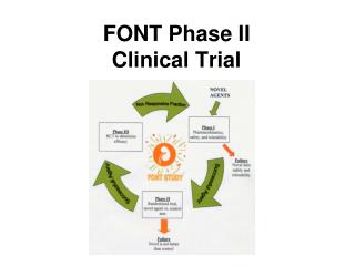
A. Background - Phase II study: Early efficacy evaluation in a “small” number of subjects There is no exact definition of ”Phase II”. There is a regulatory difference between Phases II and III. Primary Objective: • Evaluate efficacy treatment regimen • Determine whether the efficacy is adequate to warrant further testing (phase III) Secondary Objective: • Describe associated adverse events with a larger sample size than phase I trials “Phase I/II trials” test both efficacy and toxicity (don’t we always look at both?)
Endpoints • Must be quick; therefore surrogates are often used, e.g. • Response to drug (definition of “response”?) • Response Rate • Duration of response • Time to response • Progression-free survival (PFS) in cancer • Median PFS • PFS rate (e.g., 6 month PFS, 12 month PFS)
Design Requirements General requirements of a phase II study: • Short duration: • The primary endpoint should be observed early (usually excludes overall survival as a primary endpoint) • The number of available patients may be small (typically <60 patients - Strict eligibility criteria (oftentimes “second line” or “third line” patients, i.e., patients who have failed to response to standard care) • For ethical reasons, allow for early stopping if new treatment regimen is inactive (or too toxic)
Simplest form: One-arm study • It is assumed that the primary endpoint is response rate (RR) or other “good” outcome. • Design parameters: • p0: Maximum unacceptable probability of response • p1: Minimum acceptable probability of response • Scientific knowledge is derived from (statistical) hypothesis testing • Hypothesis test: H0: RR ≤ p0 vs. HA: RR ≥ p1
Simplest form: One-arm study Example: Phase II study in oncology Endpoint: Response rate Response: Response Evaluation Criteria in Solid Tumors Complete Response: Disappearance of all target lesion Partial Response: At least a 30% decrease in the sum of the longest diameter of target lesions (etc.) Overall Response Rate: Proportion of evaluable patients with CR or PR When might we consider stability a response?
Multi-stage Design • Multi-stage design: Allow for early stopping (if regimen has an unacceptably low response rate) • In a typical clinical setting it is difficult to manage more than two stages • One of the earliest two-stage designs: “Gehan’s Design” (Gehan, J Chron Dis 1961) Gehan’s Design: A preliminary trial for screening a drug for initial evidence of efficacy
Two-Stage Designs Stage 1: enroll N1 patients X1 or more respond Fewer than X1 respond Stage 2: Enroll an additional N2 patients Stop trial
B. Gehan’s Two-Stage Design • One of the earliest two-stage designs: “Gehan’s Design” (Gehan, J Chron Dis 1961) Gehan’s Design: A preliminary trial for screening a drug for initial evidence of efficacy
Typical Gehan Design • Let x% = 20% • That is, want to check if drug likely to work in at least 20% of patients 1. Enter 14 patients 2. If 0/14 responses, stop and declare true drug response 20% 3. If 1+/14 responses, add 15-40 more patients 4. Estimate response rate & C.I.
Gehan’s two-stage design: __________________________________________________ Stage 1: n1 patients are accrued: • If no response is observed, stop and declare lack of efficacy • If at least one response is observed, continue with Stage 2. • Choice of n1: Pr(No response | RR = p1) = 5% ____________________________________________ Stage 2: n2 additional patients are accrued Choice of n2: “Large enough for estimating the RR with a specified level of precision (e.g., standard error of less than 5%)”
Example: Assume that the target response rate p1 is 20% und that the desired level of precision is a standard error of less than 5%. • Choice of n1: n1= 14 is smallest integer that satisfies (the old “Rule of 14”) Pr(No response | RR = 20%) = (0.8)n1 ≤ 5% • Choice of n2: Depends on the observed RR in stage 1
Compute probability of consecutive failures: Patient Prob 1 0.8 2 0.64 (0.8 x 0.8) 3 0.512 (0.8 x 0.8 x 0.8) --- --- 8 0.16 --- --- 14 0.044 • If drug 20% effective, there would be a 1-4.4% = 95.6% chance of at least one success • If 0/14 success observed, reject drug
Gehan’s Design Sample Sizes • Stage I Sample Size Table I Rejection Effectiveness (%) Error 5 10 15 20 25 40 50 5% 59 29 19 14 11 6 5 10% 45 22 15 11 9 5 4
Stage II Sample Size • Based on desired precision of effectiveness estimate r1 = # of successes in Stage 1 n1= # of patients in Stage 1 Now precision of total sample N=(n1+ n2) Let
To be conservative, upper 75% confidence limit from first sample - Thus, we can generate a table for size of second stage (n2) based on desired precision
Additional Patients for Stage II (n2)(Rejection Rate 5% for Stage I)
Limitations of Gehan’s two-stage design: • Second stage provides no formal rule to decide whether the treatment should be tested further • No control of type I error α • Limited flexibility (e.g., type II error is fixed at 5%). • Sample size may be too large for stage 2 • Despites its limitations, Gehan’s two-stage designs are occasionally still used in practice: • In a total of 208 phase II clinical trials published in 2000, 3.3% used a Gehan’s design (Thezenas et al, European Journal of Cancer 2004)
B. SIMON Flexible Two-Stage Designs (Simon, Control Clin Trials 1989) Design Parameters: • nk: Number of patients in stage k = 1,2 • n: n = n1+ n2, maximum sample size • rk: Critical value after stage k =1,2
Simon Two-Stage Designs ____________________________________________________ • Stage 1: n1 patients are accrued: • If R1≤ r1 responses are observed, stop and conclude lack of efficacy • Otherwise, continue with Stage 2 _____________________________________________ • Stage 2: n2 additional patients are accrued: • If R ≤ r2, conclude lack of efficacy • Otherwise, conclude presence of efficacy (promising treatment, further considerations for phase III testing)
Simon’s Optimal Two-Stage Design (Simon, Control Clin Trials 1989) • How to determine (r1/n1, r2/n2)? • Subject to fixed type I error (α) and type II error (β) rates. • Appropriate type I/II error rates for phase II studies: 5% ≤ α ≤ 10% and 5% ≤β ≤ 20% • Given fixed type I error (α) and type II error (β), many designs satisfy Pr(Reject H0|RR=p0) ≥ 1 - α and Pr(Reject H0|RR=p1) ≤ β • See the following table from this paper. “PET” = “Probability of Early Termination” (e.g., after Stage 1).
Two-Stage Clinical Trials Sample Size Possible Designs For P0=0.100, P1=0.500, Alpha=0.050, Beta=0.200 Constraints N1 R1 PET N R Ave N Alpha Beta Satisfied 8 2 0.000 8 2 8.00 0.038 0.145 Single Stage 4 0 0.656 8 2 5.38 0.036 0.164 Minimax 3 0 0.729 9 2 4.63 0.041 0.172 Optimum 4 0 0.656 9 2 5.72 0.047 0.121 **Both** 4 0 0.656 10 3 6.06 0.012 0.193 **Both** 5 1 0.919 10 2 5.41 0.038 0.197 **Both** 5 0 0.590 10 3 7.05 0.013 0.178 **Both** 6 1 0.886 10 2 6.46 0.050 0.124 **Both** 6 0 0.531 10 3 7.87 0.013 0.173 **Both** 3 0 0.729 11 3 5.17 0.015 0.193 **Both** 4 0 0.656 11 3 6.41 0.017 0.145 **Both** 5 1 0.919 11 2 5.49 0.043 0.192 **Both** 5 0 0.590 11 3 7.46 0.018 0.124 **Both** 6 0 0.531 11 3 8.34 0.018 0.116 **Both** 6 1 0.886 11 3 6.57 0.015 0.163 **Both** 7 0 0.478 11 3 9.09 0.018 0.114 **Both** 7 1 0.850 11 3 7.60 0.017 0.131 **Both** 3 0 0.729 12 3 5.44 0.020 0.166 **Both** 4 0 0.656 12 3 6.75 0.022 0.113 **Both** 5 1 0.919 12 2 5.57 0.047 0.190 **Both** 5 0 0.590 12 3 7.87 0.024 0.089 **Both** 6 0 0.531 12 3 8.81 0.025 0.078 **Both** 6 1 0.886 12 3 6.69 0.019 0.140 **Both** 6 0 0.531 12 4 8.81 0.004 0.196 **Both** 7 0 0.478 12 3 9.61 0.025 0.074 **Both** 7 1 0.850 12 3 7.75 0.022 0.102 **Both**
Optimal design: Minimizes the expected sample size under H0, i.e., the assumption that the treatment has insufficient efficacy (RR= p0)
Simon’s MiniMax Two-stage Design Given fixed type I and II error rates and under the restriction Pr(Reject H0|RR=p0) ≥ 1 - α and Pr(Reject H0|RR=p1) ≤ β, MiniMax designs minimize the maximum sample size n Simon’s Optimal and Minimax Designs have been widely used in practice
Algorithm of Simon’s Method (may skip): • Early termination for non-activity Calculation of PET=Pr(stopping at stage 1|p0), where B(n, p; c) is the cumulative binomial probability of up to c events of probability p out of n subjects; individual terms are b(n,p;c) c1 =B(n1,p;c1)=∑ b(n1,p;i) i=0 • Determine n1, n2, c1 and c2 (critical values after first and second state) using a direct search method on exact probabilities Power=Pr(reject H0|p0) min(n1,c2) =1-B(n1,p,c1) - ∑ b(n1,p,m)B(n2,p;c2-m) m=c1+1
Simon’s Optimal/MiniMax designs have undesirable properties: • Optimal design with large maximum sample size n • MiniMax design with large expected sample size • Is a practical compromise possible? • Maximum sample size n close to that of MiniMax design • Expected sample size close to that of optimal design • Enumerate all designs subject to fixed type I and type II error rates • Determine a compromise between Optimal and MiniMax design using a graphical search (Jung, Carey and Kim, Control Clin Trials 2001)
Example: p0 = 30%, p1 = 50%, α = 5%, β = 15%
Balanced Design (Ye & Shyr, 2007) • Compromise between Simon’s optimal and MiniMax deign • The same number of patients are accrued for both stages (n1=n2) • Most software can compute all three designs • Balanced designs have an intuitive appeal.
Software • PASS sample size calculation software • R function ph2simon() in clinfun package > ph2simon(0.2,0.4,0.05,0.1) Simon 2-stage Phase II design Unacceptable response rate: 0.2 Desirable response rate: 0.4 Error rates: alpha = 0.05 ; beta = 0.1 r1 n1 r n EN(p0) PET(p0) Optimal 4 19 15 54 30.43 0.6733 Minimax 5 24 13 45 31.23 0.6559
D. Three-Stage Designs (Chen, Stat Med 1997) • Extension to Simon’s optimal two-stage design • Useful when accrual rate is “slow” (e.g., single institution trials) • Let PET1 denote the probability of early termination after the first stage, and PET1+2 the probability of early termination after the first or second stage • Optimal three-stage design minimizes the expected sample size under H0 (RR ≤ p0): E(n|p0) = n1 + {1 – PET1(p0)} х n2 + {1 – PET1+2(p0)} х n3
Example: p0 = 10%, p1 = 30%, α = 10%, β = 10% Three-stage optimal design Simon’s two-stage optimal design
Comparison between optimal three-stage design and Simon’s optimal two-stage design: • There is no consistent pattern for the maximum sample size (may be larger or smaller when compared to a two-stage design) • The optimal three-stage design reduces the expected sample size by an average of 10% when compared to a two-stage design
E. Phase II Designs for Multiple Endpoints • The selected primary endpoint is just one consideration in the decision to purse a new treatment • Trade-off between efficacy and toxicity: • A treatment with a high efficacy may not be of interest if too many patients experience life-threatening toxicities • A treatment with a moderate efficacy but a good toxicity profile might be still considered for future trials.
Incorporating toxicity considerations into a two-stage design (Bryant and Day, Biometrics 2001) • The toxicity profile of a new treatment undergoing phase II testing might be poorly understood: • Available phase I studies may not be directly relevant to the target patient population • The MTD of a new regimen might be very imprecise, due to small sample sizes (3-6 per dose level) in phase I studies • Bivariate extension to Simon’s optimal two-stage design: Early termination (after first stage) if: • Insufficient efficacy or • Unacceptable high toxicity rate
Response and toxicity parameters: • pR0: Maximum unacceptable probability of response • pR1: Minimum acceptable probability of response • pT0: Minimum unacceptable probability of toxicity • pT1: Maximum acceptable probability of toxicity Combined efficacy-toxicity hypothesis testing: H0R: pR≤ pR0 or H0T:pT ≥ pT0 vs. HAR: pR≥ pR1and HAT: pT≤ pT1
Sample sizes n1 and n2 and critical values for stopping are obtained by specifying three error probabilities: α, γ and 1-β: • The probability (α) of incorrectly declaring the treatment promising when the response and toxicity rates for the new therapy are the same as those of the standard therapy • The probability (γ) of incorrectly declaring the treatment promising when the response rate for the new therapy is no greater than that of the standard or the toxicity rate for the new therapy is greater than that of the standard therapy. 3. The probability (1- β ) of declaring the treatment not promising at a particular point in the alternative region
The three error probability constraints are: • Pr(XR≥cR,XT≤CT| pR=pR0,pT=pT0,θ) ≤ α 2. Sup Pr(XR≥cR,XT≤CT| pR,pT,θ) ≤ γ pR≤rR0 or PT≥pT0 3. Pr(XR≥cR,XT≤CT| pR=pRa,pT=pTa,θ) ≤ 1 - β
Design Parameters: • nk: Number of patients in stage k = 1,2 • rk: Critical value for response after stage k = 1,2 • tk: Critical value for toxicity after stage k = 1,2
Example: pR0 = 10%, pR1 = 30%, pT0 = 40%, pT1 = 20%, αR = αT = 10%, β = 10% Bivariate optimal two-stage design Simon’s optimal two-stage design
Conclusion: • Incorporating toxicity considerations into the two-stage design is useful if the toxicity profile is not fully understood • However, the cost of jointly considering both response and toxicity can be considerable (in terms of sample size requirements) • Can be modified to multivariate efficacy endpoints (e.g., response rate and 6-month PFS rate)
F. Phase II Designs for Time-to-Event Endpoints Response rate is not always a suitable primary endpoint: • Response may not always correlate strongly with survival • Challenges in response evaluation • Some promising agents are cytostatic instead of cytotoxic • Event times may be short (e.g., time to release from hospital; OS in glioblastoma multiforme)
Two-stage design for evaluating survival probabilities (Case and Morgan, BMC Med Research Meth 2003) • Assume that the primary endpoint is a survival probability, e.g., 1-year OS rate or 1-year PFS rate • Hypothesis test: H0: p ≤ p0 vs. HA: p ≥ p1 • Survival probabilities (at time x): - p0: Maximum unacceptable survival probability (at time x) - p1: Minimum acceptable survival probability (at time x) • Standard two-stage design may require inconvenient suspension of accrual at the interim analysis while patients are being followed.
Two-stage design (for x-year survival rate): Stage 1: • Accrue n1 patients until time t1. • Each patients is followed until failure or for x years or until time t1, whichever is less • If Z1(x,t1) < c1, stop the study early (lack of efficacy) • If Z1(x,t1) ≥ c1, continue with second stage Stage 2: • Accrue n2 additional patients between times t1 and t1+t2 • Each patients is followed until failure or for x years, whichever is less • If Z2(x,t1+t2) < c2: not promising regimen • If Z2(x,t1+t2) ≥ c2: promising regimen
Example:(Case and Morgan, BMC Med Research Meth 2003) Phase II study to assess the activity of a new chemo / radiation combination for patients with resectable pancreatic cancer • Primary endpoint: One-year OS rate • Hypothesis testing: H0: One-year OS rate is at most 35% vs. HA: One-year OS rate is at least 50% • Anticipated accrual rate: 24 patients per year • Type I and II error rates: α = β = 10%
Design characteristics (of design which minimizes the expected total study length):