Download

1 / 20
200 likes | 208 Views
This paper presents an optical system for resizing round flat-top distributions by imaging and resizing flat-top beams. The system is experimentally validated, showing promising results for obtaining flat-top spots at a target plane.

E N D
OPTICAL SYSTEM FOR VARIABLE RESIZING OF ROUND FLAT-TOP DISTRIBUTIONS George Nemeş, Astigmat, Santa Clara, CA, USA gnemes@astigmat-us.com John A. Hoffnagle, IBM Almaden Research Center, San Jose, CA, USA hoffnagl@almaden.ibm.com
OUTLINE 1. INTRODUCTION 2. OPTICAL SYSTEMS AND BEAMS – MATRIX TREATMENT 3. VARIABLE SPOT RESIZING OPTICAL SYSTEM (VARISPOT) 4. EXPERIMENTS 5. RESULTS AND DISCUSSION 6. CONCLUSION
1. INTRODUCTION • Importance of flat-top beams and spots • Obtaining flat-top beams • - Directly in some lasers, at least in one transverse direction • (transverse multimode lasers; excimer) • - From other beams with near-gaussian profiles – beam shapers • (transverse single-mode lasers) • Obtaining flat-top spots at a certain target plane • - Superimposing beamlets on that target plane (homogenizing) • - From flat-top beams by imaging and resizing this work
2. OPTICAL SYSTEMS AND BEAMS: MATRIX TREATMENT Basic concepts: rays, optical systems, beams Ray: R RT = (x(z) y(z) u v)
Optical system: S A11 A12 B11 B12 A B A21 A22 B21 B22 S == C D C11 C12 D11 D12 C21 C22 D21 D22 • Properties: • 0 I 1 0 0 0 • S J ST = J ; J = ; J2 = - I; I = ; 0 = • - I 0 0 1 0 0 • ADT – BCT = I • ABT = BATdet S = 1; S - max. 10 independent elements • CDT = DCT • A, D elements: numbers • B elements: lengths (m) • C elements: reciprocal lengths (m-1) • Ray transfer property of S:Rout= S Rin
Beam: P Beams in second - order moments: P = beam matrix <x2> <xy> <xu> <xv> <xy> <y2> <yu> <yv> W M W elements: lengths2 (m2) P = <RRT> = =;M elements: lengths (m) <xu> <yu> <u2> <uv> MT U U elements: angles2 (rad2) <xv> <yv> <uv> <v2> Properties: P > 0; PT= P WT= W; UT= U; MT M P - max. 10 independent elements Beam transfer property (beam "propagation" property) of S: Pout = S Pin ST W = W I Example of a beam (rotationally symmetric, stigmatic) and its "propagation" M = M I U = U I W= W0W2 = AATW0 + BBTU0 In waist: M = 0 ; Output M2 = ACT W0 + BDTU0 U = U0 plane: U2 = CCT W0 + DDTU0 Beam spatial parameters: D = 4W1/2; q = 4U1/2; M2= (p/4)D0q/l; zR = D0/q
3. VARIABLE SPOT RESIZING OPTICAL SYSTEM (VariSpot) Block diagram 3 - lens system: + cyl. lens, cyl. axis vertical ( f, 0) - cyl. lens, cyl. axis rotatable about z (-f, a) + sph. lens (f0) + free-space of length d = f0 (back-focal plane) + Cyl. (f, 0) – Cyl. (–f, α) Sph. f0 Quasi – Image Plane y x Round spot D(α) z Incoming beam D0 f0
VariSpot input-output relations W2 = W2I; W2 = A2 W0 + B2 U0 W2(a) = [(f02/f2) sin2(a)] W0 + (f02) U0 = W0 [(f02/f2) sin2(a) + f02/z2R] D(a) = D0 [(f02/f2) sin2(a) + f02/z2R]1/2 = Dm[1 + sin2(a)/sin2(aR)]1/2 Compare to free-space propagation: D(z) = Dm[1 + z2/z2R]1/2 Dm = D2(a = 0) = D0 f0 / zR = q0 f0 DM = D2(a = p/2) = D0 [(f02/f2) + f02/z2R]1/2D0 f0/ f (for f/zR <<1) sin(aR) = f/zR;aR = “angular Rayleigh range” Perfect imager B = 0 W2 = A2 W0 beam-independent “Image-mode” of optical system + incoming beam (beam-dependent - Rayleigh range zR): A2 W0 >> B2 U0 A2 >> B2/z2R f/zR = sin(aR) << sin(a) 1 VariSpot“image-mode” D(a) D0 (f0/f) sin(a)
4. EXPERIMENTS Experimental setup
Data on experiment Incoming beam data (l = 514 nm) CCD camera data (type Dalsa D7) - Gaussian beam Pixel size: 12 mm D0 = 4.480 mm Detector size: 1024 x 1024 pixels q = 0.154 mrad Dynamic range: 12 bits (4096 levels) zR = 29.1 m Noise level: 2 levels M2 = 1.05 Attenuator: Al film; OD 3 - Flat-top (Fermi-Dirac) beam D0 = 6.822 mm q = 0.149 mrad zR = 45.8 m M2 = 1.55 VariSpot data fCyl = +/- 500 mm f0 = 1000 mm a = - 900 - 00 - 900 (manually rotatable mount, +/- 0.250 resolution)
Fermi-Dirac (F-D) beam profile I(r) = I0 / {1 + exp [b (r/R0 - 1)]} R0 = 3.25 mm b = 16.25 I0 = 0.0298 mm2 M2(ideal F-D) = 1.50 M2(experimental F-D) = 1.55
5. RESULTS AND DISCUSSION Exact D(a) = D0 [(f02/f2) sin2(a) + f02/z2R]1/2 = = Dm[1 + sin2(a)/sin2(aR)]1/2 Image-mode D(a) D0(f0/f)sin(a) = DMsin(a) Gaussian beam D(a) vs. a D(a) vs. sin(a) E = dmin/dmax vs. a
Exact D(a) = D0 [(f02/f2) sin2(a) + f02/z2R]1/2 = = Dm[1 + sin2(a)/sin2(aR)]1/2 Image-mode D(a) D0(f0/f)sin(a) = DMsin(a) Flat-top (Fermi-Dirac) beam D(a) vs. a D(a) vs. sin(a) E = dmin/dmax vs. a
Estimating the zoom range in image-mode (“angular far-field”) D(a) vs. a (small angles) Kurtosis vs. a Blue lines Image-modea 40 D(a) D0(f0/f)sin(a) = DMsin(a) a 30 - 40 Zoom range in image-mode (FD FD) 13 x - 15 x
Examples of spots - Gaussian beam Incoming gaussian beam; D0 = 4.480 mm Gaussian beam in back-focal plane of f0 = 1 m spherical lens Df = 0.154 mm
Examples of spots - flat-top (Fermi-Dirac) beam Incoming Fermi-Dirac beam; D0 = 6.822 mm Fermi-Dirac beam in back-focal plane of f0 = 1 m spherical lens Df = 0.149 mm
Examples: VariSpot at working distance Gaussian beam a = 500 a = 100a = 40 Fermi-Dirac beam a = 500
Discussion - Zoom (image-mode) range (DM/Dmin) scales with zR/f - Variable spot size scales with f0 - Cheap off the shelf lenses used, no AR coating - This arrangement already shows (13 - 15) : 1 zoom range for flat-top profiles. Dmin 1.0 mm; DM 13.6 mm - Estimated (20 - 50) x zoom range for flat-top profiles - Estimated 50 mm minimum spot size with flat-top profile - Analysis smaller spots in “focus-mode”, (“Fourier-transformer-mode”, “angular near-field”) regime (not discussed here)
Prototype Zoom = 7 : 1 Dmin 1 mm; DM 7 mm
6. CONCLUSION • New zoom principle demonstrated to resize a flat-top beam at a fixed working distance • Zoom factor (dynamic range of flat-top spot sizes): (13 - 15) : 1 • Dmin1.0 mm; DM 13.6 mm • Reasonable good round spots with flat-top profiles • Estimated results using this approach (with good incoming flat-top beams and good optics): Dmin 50 mm Zoom factor: (20 - 50) : 1