Download
1 / 22
220 likes | 338 Views
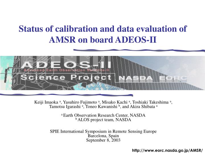
Status of calibration and data evaluation of AMSR on board ADEOS-II.

E N D
Status of calibration and data evaluation of AMSR on board ADEOS-II Keiji Imaoka a, Yasuhiro Fujimoto a, Misako Kachi a, Toshiaki Takeshima a, Tamotsu Igarashi a, Toneo Kawanishi b, and Akira Shibata aa Earth Observation Research Center, NASDAb ALOS project team, NASDASPIE International Symposium in Remote Sensing EuropeBarcelona, SpainSeptember 8, 2003
AMSR TB at all channels (path 11, January 18, 2003) 89BH 89BV 89AH 89AV 52.8V 50.3V 36H 36V 23H 23V 18H 18V 10H 10V 6H 6V
Characteristics of AMSR • Multifrequency, dual-polarized passive microwave radiometer developed by NASDA. • Higher spatial resolution compared to existing instruments (e.g., SSM/I). • Addition of 6.9-GHz channels for estimating SST and soil moisture, and 50.3 and 52.8GHz for obtaining atmospheric temperature information. • Flying in morning orbit (equatorial crossing time: 10:30 am). Combination with AMSR-E on Aqua (1:30 pm) will provide information on diurnal variability. AMSR performing conical scan measurement in orbit. Original ADEOS-II animation can be obtained from NASDA website : http://www.nasda.go.jp/
TB images of 50GHz channels First look of 52.8-GHz channel by conically scanning radiometer. 53.6GHz : ~ 4 km 52.8GHz : ~ 1 km • No limb correction is necessary. • Incidence angle of 55 degrees results in approximately 2 to 3 km of weighting peak. AMSU-A daily browse from http://pm-esip.msfc.nasa.gov/
AMSR/AMSR-E combination • Combination of AMSR-E and AMSR will be a powerful tool to investigate rapidly changing phenomena and diurnal cycle. • Cross calibration will be important to keep consistency between AMSR and AMSR-E data. Example of storm tracking by combining AMSR and AMSR-E observations. Processed by using NASDA standard algorithm developed by Dr. Petty (Univ. of Wisconsin-Madison). Rainfall rates are under validation.
Center Frequency (GHz) Bandwidth (MHz) 350 100 200 400 1000 200 400 300 Polarization Vertical and Horizontal Vertical Vertical and Horizontal 3dB Beam Width (degrees) 1.8 1.2 0.65 0.75 0.35 0.25 0.25 0.15 0.15 6.925 10.65 18.7 23.8 36.5 50.3 52.8 89.0 89.0 IFOV (km) 40x70 27x46 14x25 17x29 8x14 6x10 6x10 3x6 A B Sampling Interval (km) 10x10 5x5 Temperature Sensitivity (K) 0.34 0.7 0.7 0.6 0.7 1.8 1.6 1.2 Incidence Angle (degrees) 55.0 54.5 Dynamic Range (K) 2.7 - 340 Swath Width (km) Approximately1600 Integration Time (msec) 2.5 1.2 Quantization (bit) 12 10 Scan Cycle (sec) 1.5 Characteristics of AMSR • Non-deployable, offset parabolic antenna with effective aperture size of 2.0 m. • Total power microwave radiometers. • High Temperature noise Source (HTS) and Cold Sky Mirror (CSM) for onboard two-point calibration. • Two feed horns for 89GHz to keep enough spatial sampling in along track direction.
Direction of work • AMSR and AMSR-E are almost identical instruments in terms of radiometric characteristics. Same problem exists in HTS performance (inhomogeneous physical temperature). • Although we have to take into account the differences on thermal condition of the instruments (i.e., different local observing times), which is very important to calibration, direction of calibration activities are almost identical. • Base on discussions in course of the examination, the final calibration method may differ from the current approaches.
Radiometer sensitivity Time series of radiometric sensitivity while observing HTS (around 300K).
06V 06H 10V 10H 18V 18H 23V 23H 36V 36H 50V 52H 89AV 89AH 89BV 89BH Scan direction Sample direction (16 points for 89GHz, 8 points for others) Lunar emission in cold cal. • Moon sometimes comes insight of CSM view angle and affects the cold calibration counts sometimes up to 30K in 89 GHz due to its small beam size compare to other frequencies. • Correction is relatively straightforward since direction of the moon can be computed. After removed the affected counts, simple linear interpolation is applied to fill the gap in L1 processing system. AMSR CSM Output Voltages (March 22, 2003, Path No. 40, Ascending)
Earth emission in cold cal. • 6.925-GHz CSM counts seem to be affected by Earth’s emission (up to 1K). • Our current assumption is that this phenomena is due to a spillover occurring between feed horn and CSM. • Earth’s emission pattern is relatively unclear in AMSR case. One possible explanation is a different satellite structure that may intercept the spillover path and obscure the Earth’s emission pattern. AMSR-E AMSR Comparison of the Earth’s emission effect between AMSR-E and AMSR. Psaudo maps are made of 233 and 57 descending paths for AMSR-E and AMSR, respectively.
Land emission in cold cal. • Correlation was found between variations of contamination and Earth’s Tb of about 110 scans before. • L1 processing system subtract this contamination by assuming CSM spillover (spillover occurring between feed horn and CSM) Spillover factor was statistically found and used for correction. Before After Sample images showing the correction. Maps are made of 57 descending paths.
Radiometric correction Step 1 : PRT method Step 2 : RxT method • Multiple regression model of Teff using eight PRT readings. • Coefficients of the regression model were determined by using SSM/I oceanic Tb (18GHz and higher channels) and computed Tb (6 and 10GHz channels) based on the Reynolds OI-SST analysis. SSM/I data were provided by the Global Hydrology Resource Center (GHRC) at the Global Hydrology and Climate Center, Huntsville, Alabama, USA. Reynolds OI-SST dataset were made available by NOAA. • Utilize Relationship between receiver temperature and its gain variation. • Applying this equation to HTS measurement and assuming Teff derived by regression model as TOBS, bRX can be computed by regression analysis. Using this value, gain variations can be compensated by the equation. HTS Effective Temp. PRT readings TOBS : Scene Tb (K) TCSM : Deep space Tb (K) C’OBS : Digital counts of scene C’CSM : Digital counts of deep spece G0 : Nominal gain bRX : Gain sensitivity to rec. temp. (℃-1) DTRX : Rec. temp. departure from mean value (℃).
HTS effective temperature Ta HTS Temp. (target) TH SSM/I or simulated Earth Tb TOBS Deep space Temp. TC Counts CC COBS CH AMSR-E measurement Extrapolating HTS effective temperature (target) by using Earth Tb
Combining PRT and RxT From PRT method 23GHz Vpol Tb_HTS & Treciever
Improvement by adding RxT method BLUE :HTS effective temp. by PRT method. RED:HTS effective temp.by PRT+RxT method. RED:Difference between above two.
Radiometric correction6.925GHz tentative results Comparison between computed Tb based on OI-SST and AMSR Tb by (a) simple two-point calibration and (b) presented method for 6.925-GHz vertical polarization on June 3, 2003. (c) Daily average of difference between computed and AMSR Tb as a function of position in orbit for simple two-point calibration (cross) and presented method (closed circle).
Radiometric correction36.5GHz tentative results Comparison between SSM/I Tb (corrected for difference of incidence angle and center frequency) and AMSR Tb by (a) simple two-point calibration and (b) presented method for 36.5-GHz vertical polarization on June 3, 2003. (c) Daily average of difference between SSM/I Tb and AMSR Tb as a function of position in orbit for simple two-point calibration (cross) and presented method (closed circle).
AMSR and AMSR-E comparison It should be noted that AMSR TB are still tentative version.
6.925GHz RFI 6.925GHz vertical polarization, ascending passes (July 8, 2003)
Known issues and on-going works • Possible overestimation in high Tb over land in 6.925 GHz. Suspect receiver non-linearity characteristics. • Need further improvement particularly at lower frequency channels (for SST, etc.). • Comparison of 50GHz channels TB with AMSU TB with an incidence angle of near 55 degrees. • Utilization of SeaWinds wind speed data to minimize the uncertainties in comparing AMSR TB and computed TB based on Reynolds-SST. • Comparison of AMSR and AMSR-E to keep these data set consistent. • Assessment of other systematic errors (e.g., scan bias). • Assessment of geolocation errors (errors may not be corrected if its size does not exceeds that of AMSR-E).
Summary and conclusions • AMSR is providing stable data stream since the beginning of normal operation. • Same approaches (that were applied to AMSR-E) of post-launch evaluation and calibration are being tested. Some preliminary results of calibration were presented. • Our current target date of releasing the data is after 1-year from ADEOS-II launch.
AMSR-E data status • NASDA/EOC started distribution of AMSR-E L1 brightness temperature (and L3-Tb) products from June 18, 2003. • http://www.eoc.nasda.go.jp/amsr-e/index_e.html • http://www.eorc.nasda.go.jp/AMSR → AMSR-E Data Release • L1A (raw counts) data are also available at NSIDC. • http://nsidc.org → Data catalog → AMSR-E/Aqua L1A Raw Observation Counts