Download
1 / 14
160 likes | 233 Views
Solution of ODEs by Laplace Transforms. Procedure: Take the L of both sides of the ODE. Rearrange the resulting algebraic equation in the s domain to solve for the L of the output variable, e.g., Y ( s ). Perform a partial fraction expansion.

E N D
Solution of ODEs by Laplace Transforms • Procedure: • Take the L of both sides of the ODE. • Rearrange the resulting algebraic equation in the s domain to solve for the L of the output variable, e.g., Y(s). • Perform a partial fraction expansion. • Use the L-1 to find y(t) from the expression for Y(s).
Example 3.1 Solve the ODE, First, take L of both sides of (3-26), Rearrange, Take L-1, From Table 3.1,
Example 2: system at rest (s.s.) Chapter 3 To find transient response for u(t) = unit step at t > 0 1. Take Laplace Transform (L.T.) 2. Factor, use partial fraction decomposition 3. Take inverse L.T. Step 1Take L.T. (note zero initial conditions)
Rearranging, Step 2a. Factor denominator of Y(s) Chapter 3 Step 2b. Use partial fraction decomposition Multiply by s, set s = 0
Partial Fraction Expansions Basic idea: Expand a complex expression for Y(s) into simpler terms, each of which appears in the Laplace Transform table. Then you can take the L-1 of both sides of the equation to obtain y(t). Example: Perform a partial fraction expansion (PFE) where coefficients and have to be determined.
To find : Multiply both sides by s + 1 and let s = -1 To find : Multiply both sides by s + 4 and let s = -4 A General PFE Consider a general expression,
Here D(s) is an n-th order polynomial with the roots all being real numbers which are distinct so there are no repeated roots. The PFE is: Note:D(s) is called the “characteristic polynomial”. • Special Situations: • Two other types of situations commonly occur when D(s) has: • Complex roots: e.g., • Repeated roots (e.g., ) • For these situations, the PFE has a different form. See SEM • text (pp. 61-64) for details.
Example 3.2 (continued) Recall that the ODE, , with zero initial conditions resulted in the expression The denominator can be factored as Note: Normally, numerical techniques are required in order to calculate the roots. The PFE for (3-40) is
Step 2b. Use partial fraction decomposition Multiply by s, set s = 0 Chapter 3
For a2, multiply by (s+1), set s=-1 (same procedure for a3, a4) Step 3.Take inverse of L.T. Chapter 3 You can use this method on any order of ODE, limited only by factoring of denominator polynomial (characteristic equation) Must use modified procedure for repeated roots, imaginary roots
Solve for coefficients to get (For example, find , by multiplying both sides by s and then setting s = 0.) Substitute numerical values into (3-51): Take L-1 of both sides: From Table 3.1,
Important Properties of Laplace Transforms • Final Value Theorem It can be used to find the steady-state value of a closed loop system (providing that a steady-state value exists. Statement of FVT: providing that the limit exists (is finite) for all where Re (s) denotes the real part of complex variable, s.
Example: Suppose, Then, 2. Time Delay Time delays occur due to fluid flow, time required to do an analysis (e.g., gas chromatograph). The delayed signal can be represented as Also,