Download
1 / 49
490 likes | 499 Views
Introduction to Observational Physical Oceanography 12.808 Class 6, 29 September 2009 these slides are available online at http://www.whoi.edu/science/PO/people/jprice/class/miscart/Class6-29Sep09.ppt. Class 6. Last time -T/S Diagrams -Water types and masses

E N D
Introduction to Observational Physical Oceanography 12.808 Class 6, 29 September 2009 these slides are available online at http://www.whoi.edu/science/PO/people/jprice/class/miscart/Class6-29Sep09.ppt
Class 6 • Last time • -T/S Diagrams • -Water types and masses • This week--Topic 3: Anthropogenic and biologically active tracers • Non-conservative Tracers – O2, preformed phosphate • Transient Anthropogenic Tracers – CFCs Recommended reading: Secs. 1 and 2 of Gruber and Sarmiento 2002
REMINDER HW #3 part 1 3.1) Help us figure out where the five mystery stations, Amysterystas2009.mat, were taken. Major hint – somewhere in the Atlantic. Use T/S properties to figure out what basin the station must have been in. To load these mystery station data into Matlab, see readme_hydrography.m . You will need to edit the input data file name, and make a T/S diagram. May be helpful to annotate the T/S diagram with the major Atlantic water types. This will be due Oct 8 (next Thursday).
AAIW Med NADW AABW Med AAIW NADW AABW
TOPIC 3 - Tracers • Other tracers, in addition to T and S, provide us with crucial • additional information on the ocean circulation, its time scales • as well as the exchange with the atmosphere and ocean life. • 1)Biologically active tracers; dissolved oxygen, • nitrogen as nitrate, NO3- , and phosphorous as • phosphate, PO43-. These tracers are not conserved. • 2) Anthropogenic tracers – transient tracers • CFCs, tritium, Carbon-14 • 3)NaturalRadioactive trace elements; uranium and thorium. • Good basic references are Ocean Chemistry, 1989 Ch.2 • and the first 1/3 of Gruber and Sarmiento, The Sea, 2002.
Biologically active, non-conservative tracers Biologically active tracers – e.g. nutrients, dissolved oxygen, DIC (dissolved inorganic carbon), preformed phosphate - the surface value is modified by biological sources and sinks.
Biologically active, non-conservative tracers The Soft Tissue Pump (Volk and Hoffert, 1985) Surface Ocean Dissolved oxygen Particulate org. matter Dissolved org. matter light nutrients CO2 Photosynthesis Deep Ocean Remineralization (respiration, Decomposition) nutrients CO2 Dissolved oxygen organic matter
The Conveyor Belt biological material Broecker and Peng, ‘88
Biologically active, non-conservative tracers Photosynthesis in the upper ocean produces organic material, depletes nutrients and releases oxygen Organic particles fall into the deep ocean Decomposition or respiration occurs in the deep ocean, releases nutrients, consumes oxygen Ocean Chem 89
respiration respiration afterOcean Chem 89 0 280 dissolved oxygen mmol kg-1
Dissolved Oxygen Concentration • Sources • the atmosphere through air-sea gas exchange • 2) Photosynthesis in the surface ocean • Sinks • 1) Respiration/remineralization
Atmospheric Oxygen Solubility Like CFCs – solubility is a strong function of temperature Osat = sw_satO2(S,T) units are ml l-1 Units: older unit: ml l-1 modern unit: mmolkg-1 ml l-1 x 43.1 = mmol kg-1 X100 = mmol kg-1
Phosphate Concentration—a nutrient! • Sources • Respiration/remineralization • Runoff Sinks 1) Photosynthesis
The Conveyor Belt biological material Broecker and Peng, ‘88
O-4000 3.2 6.2 3.6 4.0 4.4 5.4 5.6
Apparent Oxygen Utilization AOU = Osaturation(S,T) – Oobserved shows how much oxygen has been depleted by respiration, independent of the temperature effect upon saturation. A note regards units: our seawater routine, sw_satO2(S, T), returns the old units, ml/l (milliliters per liter); to convert to the new units, micro moles/ kg, multiply by 43.1
AOU ~ how much oxygen has been used by respiration AOU-4000 1.2 4.8 NADW 4.0 3.8 PCW 2.4 PCW 3.2 2.8 AABW + AAIW
dissolved oxygen concentration Units: older unit: ml l-1 modern unit: mmolkg-1 ml l-1 x 43.1 = mmol kg-1 Osat = sw_satO2(S,T) units are ml l-1 X100 = mmol kg-1 In the surface layer, oxygen is released by photosynthesis and exchanged with the atmosphere; the latter is an infinite source/sink, and drives the ocean surface layer to saturation in a time scale of O(10 days).
Most organic matter seems to be made up from a nearly constant ‘recipe’ of the basic elements: the Redfield Ratios during respiration P goes up while O2 goes down and with a more less constant ratio, P:O2 = 1:170 +- 10 from Gruber and Sarmiento, 2002
Preformed Phosphate, Ppre = Pobs - Premin is a quasi-conservative tracer of deep water circulation Pobs is the observed phosphate Premin is the Phosphate that has been added by respiration Premin = AOU/170, where 1:170 is the Redfield ratio of phosphorus to dissolved oxygen Some crucial data - the boundary conditions on deep values of Ppre are observed to be: Ppre of NADW = 0.8 (+-0.1) Ppre of AABW and AAIW = 1.5 (+-0.1) Deep water is a mixture of these two end members; by calculating Ppre we can infer the fraction of northern and southern waters (in deep waters).
from Gruber and Sarmiento, The Sea, 2002 The first two sections are very highly recommended.
Preformed Phosphate 1.5 0.8 NADW AABW
Transient, anthropogenic (man-made) tracers 1) CFCs, inert chemicals that can be detected in minute amounts. They make a nearly perfect ‘dye’. 2) radioactive tracers from nuclear bomb testing: tritium, carbon 14, and others.
CFCs have been produced (and released) into the atmosphere since about 1960: from Fine, EOS, 2001
Air-Sea Gas Exchange • From high to low concentration • gas exchange rate depends on many factors: wind speed, waves, ice-cover, mixing, surfactants • Depends on solubility (which in turn depends on temperature), typically increases at lower temperatures • Depends on concentration
CFCs: • High atmospheric concentration, low oceanic • Equilibrium (~ days) is reached when the ocean is saturated in CFCs • higher solubility in cold waters • USES: • Inert dye for the ocean circulation with a time-dependent input function • Useful to determine timescales, variability and age of water parcels • Analog to CO2 with the advantage of being biologically and chemically inert
CFCs in the Atlantic – Meridional Section www.ewoce.org
Ages in the Ocean Tracer age – time since a parcel was last at the surface Fine et al. 2002
North Pacific Western North Atlantic Fine, EOS