Download
1 / 38
380 likes | 385 Views
Learn the basics of 1st level data analysis in SPM5, including design matrix specification, GLM parameter estimation, and result interpretation using contrasts.

E N D
1st level analysis - Design matrix, contrasts & inference Nico Bunzeck, Katya Woollett
1st level data analysis in SPM5 • (i) Specification of the GLM design matrix, fMRI data files and filtering • (ii) estimation of GLM parameters using classical or Bayesian approaches • (iii) interrogation of results using contrast vectors to produce Statistical Parametric Maps (SPMs) or Posterior Probability Maps (PPMs)
(i) fMRI model specification • Timing parameters: to construct the design matrix • Units for design: onset of the events or blocks (in sec or scans) • Interscan interval: TR in sec; = time between acquiring a plane for one volume and the same plane in the next volume; constant • Microtime resolution: (t) the number of time-bins per scan used when building the regressors (default = 16) • Microtime onset: (t0) the first time-bin at which the regressors are resampled to coincide with data acquisition (default = 1)
(i) fMRI model specification • Data & Design matrix: defines the experimental design and the nature of the hypothesis testing • matrix: organized in rows (each scans) and columns (for each effect of explanatory variable = regressor or stimulus function) • can be replicated and/or manipulated for each subject/session
(i) fMRI model specification • Subjects/Session: • Scans: select the images for the model that has to be estimated
(i) fMRI model specification • Condition: can be event-related, blocked design or a combination of both – they are modelled in the same way -> they are later convolved with a basis set • - Name: be creative • Onset: specify the onsets for this condition • Durations: default for events = 0; single number: SPM assumes that all trails have this duration (block) • for mix of blocks and events: number must match the number of onset times
(i) fMRI model specification • Multiple conditions: • load all the conditions defined as *.mat • it contains cell arrays: names, onsets and duration eg. Names{2}=‘finger tapping’, onsets{2}=[10 45 100], duration{2}=[0 0 0]
(i) fMRI model specification • Regressors: additional columns in the design matrix that may not be convolved with the HR, eg. movement parameters • Name • Value • Multiple regressors: either *.mat or *.txt file that contains details of the multiple regressors; they will be named: R1, R2 … Rn
(i) fMRI model specification • High-pass filter cutoff: default = 128s • slow signal drifts with a period longer than 128 will be removed • removes confounds without estimating their parameters explicitly
(i) fMRI model specification • Factorial design: if you have a factorial design SPM automatically generate the contrasts that are necessary to test the main effects of interaction: • F-contrasts: at within-subject level • contrasts for second level analysis • create as many factors as you need – name, levels (for each factor) • for example: ‘Stimulus-Repetition’ – 3 levels
(i) fMRI model specification • Basis Functions: • SPM uses basis functions to model the hemodynamic response; either 1 function or a set • Canonical HRF: most common choice, default, easiest way to interpret the data • Model derivatives: = ‘informed’ basis set -> covers variations in subject-to-subject and voxel-to-voxel responses: peak and width
(i) fMRI model specification • Model interactions: inputs (RT) convolved with the basis set • Directory: where the SPM.mat file will be written
(i) fMRI model specification • Global normalization: • estimating the ‘average within-brain fMRI signal’ (gns) over scans (n) and sessions (s) • ‘Scaling’: SPM multiplies each value in scan and session by 100/(gns) eg. scaling over all sessions • ‘none’: default, estimation of a ‘session specific grand mean value’ (gs) = fMRI signal over all voxels in a session; each fMRI data point in the session is multiplied by 100/(gs); eg. Session specific scaling
(i) fMRI model specification • Explicit masking: only those voxels in the brain mask will be analyzed • speeds up the estimation • restricts SPMs to within-mask voxels • Serial correlations: due to aliased biorhythms and unmodelled neural activity • SPM uses an autoregressive AR(1) model during Classical (ReML) parameter estimation • but they can be ignored (‘none’) - Bayesion estimation
(i) fMRI model specification • What should be included in the model? • Think about contrast/comparisons before the experiment • The more information you have the better: the model represents the a priori ideas about how the experimental paradigm influences the measured signal
(i) Review a specified model • Design matrix: • 24 conditions/session • last 2 columns model average activity in each session -> total of 50 regressors • 191 fMRI scans/session -> 382 rows and 50 columns
(i) Review a specified model • Explore Sessions and regressors: • time domain corresponding to the regressor (4 events) • frequency domain corresponding to the regressor: experimental variance is not removed by high-pass filtering • bottom: basis function = HRF
(ii) fMRI model estimation • for which voxel does the model (or a explanatory variable) explain the observed variance?? • parameters are estimated for each voxel so that the error is minimized • there are more than 1 variables -> it is unlikely that the betas exactly fit: SPM calculates different parameter-sets • each parameter-set determines a fitted response: • differs slightly from the observed Yj • the algorithm minimizes the residuals
(ii) fMRI model estimation Fitting X to Y gives you one (parameter estimate) for each column of X and e. Betas provide information about the fit of the regressor X to the data, Y, in each voxel
(ii) fMRI model estimation • Select SPM.mat: - • Method: • “Classical”:applies Restricted Maximum Likelihood (ReML); for spatially smoothed images • after estimation effects of parameters are tested by T and F-statistic -> SPM(T), SPM(F) • “Bayesian 1st-level”:applies Variational Bayes (VB); images do not need to be spatially smoothed; takes long; • results: contrasts identify regions with effects larger than a user-specified size, eg 1% of the global mean signal (Posterior Probability Map – PPM)
(iii) Results • Testing hypothesis • T-test: is there a significant increase or is there a significant decrease in a specific contrast (between conditions) – directional • F-test: is there a significant difference between conditions in the contrast - nondirectional
T-Contrast: (iii) Results • Contrast-vector:c‘= [-1 1 0 0 0 0 ] • H0: no difference between condition 1 and 2 in the 1st block • H1: there is a difference between condition 2 and 1 in the 1st block (condition 2 > condition 1) Parameters: Design matrix: T-statistics in the usual way: Comparison of betas to variance
(iii) Results • Contrast-vector:c‘= [-1 1 -1 1 0 0 ] • H0: no difference between condition 1 and 2 in the 1st and 2nd block • H1: there is a difference between condition 2 and 1 in the 1st and 2nd block (condition 2 > condition 1) T-Contrast: Parameters: Design matrix: T-statistics in the usual way: Comparison of betas to variance
(iii) Results • Contrast-vector:c‘= [1 0 0 0 0 0 0; • 0 1 0 0 0 0 0; • 0 0 1 0 0 0 0; • 0 0 0 1 0 0 0; • 0 0 0 0 1 0 0] • H0: the factors 1, 2, 3 and 4 do not explain a significant amount of variance • H1:the factors 1, 2, 3 and 4 do explain a significant amount of variance: F-Contrast: Parameters: Design matrix:
(iii) Results • Contrast-vector:c‘= [1 0 0 0 0 0 0; • 0 0 0 0 0 0 0; • 0 0 0 0 0 0 0; • 0 0 0 0 0 0 0; • 0 0 0 0 0 0 0] • H0: the factor 1 does not explain a significant amount of variance • H1:the factor 1 does explain a significant amount of variance: F-Contrast: Parameters: Design matrix:
(iii) Results Results: Glas-brain (maximum intensity projection (MIP)) List of activated voxel
The multiple comparison problem Voxel-level P: chance of finding a voxel with this or a greater height (T or Z), corrected or uncorrected for search volume Uncorrected: Default: 0.001 -> 50.000 voxels = 50 false positives FWE: ‘family wise error’ is a false positive anywhere in theSPM controls any false positives FDR: ‘false discovery rate’ – controls the expected proportion of false positives among suprathresholded voxels -> it adapts to the amount of signal in the data (iii) Results Results: Glas-brain (maximum intensity projection (MIP)) List of activated voxel
(iii) Results Results: Glas-brain (maximum intensity projection (MIP)) List of activated clusters corrected uncorrected
(iii) Results • Cluster level (P): chance of finding a cluster with this many (ke) or a greater number of voxel, corrected or uncorrected for search volume • Set-level (P): the chance of finding this (c) or a greater number of clusters in the search volume Results: Glas-brain (maximum intensity projection (MIP)) List of activated clusters corrected uncorrected
(iii) Results Plotting responses Estimated effect sizes Fitted responses
(iii) Results Overlaying the data Slices Sections
(iii) Results Overlaying the data Render
(ii) fMRI model estimation • Bayesian 1st-level: applies Variational Bayes (VB); allows to specify spatial priors for regression coefficients and regularised voxel-wise AR(P) modelsfor fMRI noise prcesses • images do not need to be spatially smoothed • takes 5x longer than the classical approach • results: contrasts identify regions with effects larger than a user-specified size, eg 1% of the global mean signal (Posterior Probability Map – PPM)
Matrix design Graphical design (ii) fMRI model estimation