Download
1 / 24
240 likes | 256 Views
Assessing Association Strength and Causation. October 14 2004 Epidemiology 511 W.A. Kukull. Assumption. “ We can draw an inference about the experience of an entire population based on the evaluation of only a sample.” (H&B)

E N D
Assessing Association Strength and Causation October 14 2004 Epidemiology 511 W.A. Kukull
Assumption • “ We can draw an inference about the experience of an entire population based on the evaluation of only a sample.” (H&B) • If we draw many samples from the same population, to determine the proportion of 70+ year old men with hip replacement • the estimate will vary from sample to sample • larger samples will have less variability
Statistical Association and chance • Does “sample” association represent “population” association? • Luck of the draw • Uneven distribution of factor • Smaller sample => more variability • The “null” hypothesis • Factor X is not associated with Disease Y
Good-bye Intraocular ImpactTest • We can’t always tell just by “looking” • We need statistics (believe it or not) • to evaluate the true vs. chance observation • to adjust for extraneous “other” effects • to examine changes in association across categories of another factor • to determine whether we might have missed a true effect
Acceptable levels • Statistical tests let us set the “chance” level • alpha level : convention .05 • the observed association could have occurred, due to chance alone, < 5% of the time [when there was really no true association between E and D] • Type I error : we would erroneously conclude there is a true association, when it was really only due to chance. • can be set at a lower or higher level : 0.0001
Reality Not assoc. Associated Type II Error Not Assoc. Correct Observation (beta) Type I Error Correct Associate (power) (alpha) Are they Associated?
Careful what you say... • Statistical significance • does not mean chance cannot have accounted for the finding -only that it is unlikely • non-significance does not mean chance is the reason for lack of association • provides no information about adequacy of the design, potential bias or (usually) confounding • non-significance does not mean there can be no causal association --it could be a small sample
More caution:“The glitter of the t-table diverts attention from the inadequacy of the fare.” --A.B. Hill • Statistical significance • does not address whether differences are important to health • does not indicate biologic plausibility • may not reflect clinical relevance • Confidence intervals give us more information than p-values alone
Relative risk “estimates” Increasing risk Decreasing risk (protective) Zero Infinity 1.0 “Null” lower incidence in exposed or fewer exposed among cases higher incidence in exposed or more exposed among cases
Confidence Intervals(non-computational view) • We calculated the RR, but how good is it? • The true measure of effect lies between these bounds, with X% confidence • “we are 95% sure that the true odds ratio lies between 1.2 and 6.7” • Small sample size may be inadequate to exclude chance as an explanation
Confidence IntervalsWhat they tell us • Wider intervals indicate smaller sample size, lack of precision, low power • Narrower intervals indicate greater precision • More information than a p-value alone • If they do not include the “null value” (1.0 for RR) => “statistical significance”
2 x 2 table “Case-Control” Study Case Control a b Exposed Not Exposed c d Odds Ratio = (ad) / (bc)
Confidence Interval for Odds Ratio (Unmatched case-control study) ] (ad)/ (bc) exp[+ z confInt = var (ln OR) 1/a + 1/b + 1/c + 1/d z = normal curve value z = 1.96 corresponds to 95% confidence (2.58 corresponds to 99% confidence)
Case Control 32 825 Exposed Not Exposed 56 1048 Odds Ratio = (ad) / (bc) = 0.73
OR = 0.73 +z 1/a + 1/b + 1/c + 1/d (OR) exp + 1.96 (1/32 + 1/825 + 1/56 + 1/1048) (OR) exp + 0.44 Then 95% CI = (0.73) e+ 0.44 LL = (0.73) (0.64) = 0.47 } 0.47 – 1.13 UL = (0.73) (1.55) = 1.13
Easy definitions • “e” represents the base of the natural log scale; you can usually find it on calculators • “exp” indicates you are to raise “e” to a power: • exp (0.44) means e0.44 • exp (-0.44) means e -0.44 • this is often described as taking the “antilog” • Try it on a calculator, real easy
Confidence Interval for Odds Ratio (Matched study) ] (b/c) exp[+ z ConfInt = var (ln OR) 1/b + 1/c z = normal curve value z = 1.96 corresponds to 95% confidence (2.58 corresponds to 99% confidence)
Confidence Interval for Cohort (Cumul.incidence type) ] RR exp[+ z Conf. Int = var (ln RR) {b/ a(a+b)} +{d/ c(c+d)} z = normal curve value z = 1.96 corresponds to 95% confidence (2.58 corresponds to 99% confidence)
Bias • Flaws in the design and conduct of a study • Were subjects for comparison groups selected by different means relative to exposure or disease • Selection bias • Was information gathered in a different way from subjects of one group relative to the other • Interviewer bias • Recall bias
Confounding • Effect of interelations between known or unknown study variables: mixing effects • Is there a third factor associated with both exposure and disease (e.g., another risk factor) that alters the observed effect? • true association may be stronger or weaker • ? Coffee drinking => pancreatic Ca • smoking associated with both?
Summary • Is the statistical association valid? • Due to Chance? • Due to Bias? • Due to Confounding?
Validity and Generalizability • Validity (internal) must be primary objective--invalid results are not generalizable • “ but your subjects aren’t representative of the entire population…” . • it’s more important to have subjects who are comparable on other risk factors, and can supply complete & accurate information • Consider: Nurses Health study; British physicians study, Framingham
Summary (2) • If valid, is the association causal ? • strong association • biologic plausibility • consistency • time sequence • dose-response relationship