D S R

1. Communications Analytics prediction and anomaly detection for emails, tweets, phone, text fR 0 0 0 0 0 0 0 0 0 fR 0 0 0 fS f1,S f2,S 0 0 0 0 1 1 1 1 0 0 0 0 1 1 1 1 0 0 0 0 0 0 0 0 0 0 0 0 1 1 1 1 0 1 0 1 1 1 1 1 0 0 0 0 1 1 1 1 0 0 0 0 0 0 0 1 0 0 0 0 0 0 0 0 0 0 0 0 1 1 1 1 DSR 2 3 4 0 1 0 1 fS 5 T TD 0 fD fU fT 0 1 1 0 0 0 0 0 1 1 1 1 1 0 0 0 0 0 0 0 0 0 2 2 0 0 1 1 1 1 1 1 0 0 0 3 3 1 0 0 1 fD 0 0 0 0 0 0 4 4 fT 5 5 0 fT fD D D 0 1 0 0 1 1 0 0 1 1 2 2 0 0 0 0 0 0 0 1 1 2 3 3 3 UT 4 4 4 5 5 0 1 0 0 5 0 1 0 1 fD U U 0 0 0 1 T 0 0 1 0 0 0 0 1 Use GradientDescent+LineSearch to minimize sum of square errors, sse, where sse is the sum over all nonblanks in TD, UT and DSR. Should we train User feature segments separately (train fU with UT only and train fS and fR with DSR only?) or train U with UT and DSR, then let fS = fR = fU , so f = This will be called 3D f. FU 0 0 0 1 0 1 0 0 1 0 1 1 0 0 1 1 0 1 0 1 0 1 1 <----fT----> <----fR----> <----fS----> <----fU----> <----fD----> 0 Or training User the feature segment just once, f = This will be called 3DTU f 0 1 0 1 0 1 0 1 0 1 0 1 <----fT----> <----fD----> <fU=fS=fR> 0 1 0 1 fT Using a 3-dim DSR(Document Sender Receiver) matrix and 2-dim TD(Term,Doc) and UT(User Term) matrixes. The pSVD trick is to replace these massive relationship matrixes with small feature matrixes. Using just one feature, replace with vectors, f=fDfTfUfSfRor f=fDfTfU rec DSR  sender  Replace DSR with fD, fS, fR TD Replace TD with fT and fD UT Replace UT with fU and fT feature matrixes (2 features) We do pTrees conversions and train F in the CLOUD; then download the resulting F to user's personal devices for predictions, anomaly detections. The same setup should work for phone record Documents, tweet Documents (in the US Library of Congress) and text Documents, etc.

2. pDTT1,0 pTDD2,1 pTUU1,2 pTDD2,0 pDRMask pDTT1,2 pTDD2,Mask pUTT3,1 pUTT2,0 pUTT2,1 pRDD2,1 pUTT2,2 pUTT2,Mask pRDD1,2 pRDMask pUTT1,2 pUTT1,0 pDCT,1 pUTT1,1 pUTT3,0 pUTT1,Mask pUTT3,2 pTDD2,2 pTUU1,1 pUTT2,Mask pTDD1,0 pTDD1,Mask pDLN,1 pDRR2 pDTT2,2 pDTT2,1 pDRR1 pDTT2,0 pDTT2,Mask pTUU2,Mask pDTT1,Mask pDTT3,2 pDTT1,1 pTUU1,0 pDTT3,1 pDTT3,0 pTUU2,1 pDTT3,Mask pTUU2,2 pDS,1 pTUU1,Mask pTDD1,2 pTDD1,1 pTUU2,0 0 1 0 1 0 1 0 0 0 0 0 0 0 0 1 1 0 1 0 0 1 1 1 0 0 0 0 1 1 0 1 0 1 0 1 1 0 0 1 0 0 1 0 0 1 0 1 0 1 0 1 0 0 1 0 1 0 1 1 1 1 0 1 1 1 1 0 1 0 0 1 0 1 1 1 1 1 0 1 1 1 1 1 1 1 0 0 0 0 1 1 1 0 0 1 1 1 1 1 1 1 0 0 0 1 1 0 0 1 1 0 1 1 0 TU RD TD 1 3 1 4 1 1 5 5 0 1 2 3 4 1 pDSh,0 pDCT,0 pDLN,0 1 1 1 0 1 0 DT 4 5 1 3 3DTU: Structure relationship as a rotatable matrix, then create PTreeSets for each rotation (attach entity tbl PTreeSet to its rotation Always treat an entity as an attr of another entity if possible? Rather than add it as a new dimension of a matrix? E.g., Treat Sender as a Document attribute instead of as the 3rd dim of matix DSR. The reason: Sender is a candidate key for Doc (while Receiver is not). (Problem to solve: mechanism for SVD prediction of Sender?) DR SenderCTLN 1 3 1 2 1 2 1 0 1 1 1 2 D 1 2 3 T UT U 1 3 5 4 2 1 2 1 Only provide blankmask when blanks pTrees might be provided for DST (SendTime) and D(LN (Length):

3. Here we try a comprehensive comparison of the 3 alternatives, 3D (DSR); 2D (DS, DR); DTU(2D) [em9 em10] DT 1 3 4 5 UT 3 5 4 u1 1 2 1 u2 DSRs1 s2 s1 s2 1 d1 r1 d1 r2 1 d2 1 d2 1 1 1 1 1 1 1 1 1 1 1 sseDTU 65.066 tDSU 1.12 T1 T2 T3 D1 D2 U1 U2 S1 S2 R1 R2 sse2D 59.455 t2D 1.24 1.0 1.0 1.0 1.0 1.0 1.0 1.0 1.0 1.0 1.0 1.0 sse3D 64.380 t3D 1.09 4.6 9.1 4.8 -3. 3.4 9.1 0.4 -3. -4. -3. -4. sseDTU 60.875 tDSU 0.025 T1 T2 T3 D1 D2 U1 U2 S1 S2 R1 R2 sse2D 19.197 t2D 0.11 1.6 2.2 1.7 0.6 1.5 2.2 1.1 0.6 0.4 0.6 0.4 sse3D 13.877 t3D 0.129 -0. 1.1 0.3 2.8 6.0 -1. -4. 0.4 -0. 0.2 -0. sseDTU 60.841 tDSU -0.001 T1 T2 T3 D1 D2 U1 U2 S1 S2 R1 R2 sse2D 15.334 t2D 0.086 1.5 2.4 1.7 0.9 2.1 2.0 0.6 0.6 0.3 0.6 0.4 sse3D 6.0480 t3D 0.11 -0. -0. 1.8 0.9 0.2 -0. 0.8 0.4 -1. -0. -0. sseDTU 60.808 tDSU -0.002 T1 T2 T3 D1 D2 U1 U2 S1 S2 R1 R2 sse2D 14.196 t2D 0.07 1.5 2.3 1.9 1.1 2.2 2.0 0.7 0.7 0.2 0.5 0.2 sse3D 5.1468 t3D 0.121 -0. -0. 0.2 0.1 0.3 -0. -0. 0.4 -0. -0. -0. sseDTU 60.806 tDSU -0.001 T1 T2 T3 D1 D2 U1 U2 S1 S2 R1 R2 sse2D 14.151 t2D -0.015 1.5 2.3 1.9 1.1 2.2 2.0 0.7 0.7 0.1 0.5 0.2 sse3D 5.0888 t3D 0.06 DT 1 3 4 5 UT 5 5 u1 5 u2 DSR s1 s2s1 s2 1 d1 r1 d1 r2 d2 1 d2 1 1 1 1 1 1 1 1 1 1 1 sseDTU 65.198 tDSU 1.1 T1 T2 T3 D1 D2 U1 U2 S1 S2 R1 R2 sse2D 85.339 t2D 1.2 1.0 1.0 1.0 1.0 1.0 1.0 1.0 1.0 1.0 1.0 1.0 sse3D 88.579 t3D 1.06 5.8 7.0 4.9 -1. 1.8 7.0 1.7 -4. -4. -4. -4. sseDTU 59.968 tDSU 0.028 T1 T2 T3 D1 D2 U1 U2 S1 S2 R1 R2 sse2D 21.766 t2D 0.14 1.8 2.0 1.7 0.8 1.3 2.0 1.3 0.4 0.4 0.4 0.4 sse3D 47.721 t3D 0.14 0.6 1.2 -2. 1.5 7.4 -2. -5. 0.0 -0. 0.1 -0. sseDTU 59.934 tDSU -0.001 T1 T2 T3 D1 D2 U1 U2 S1 S2 R1 R2 sse2D 13.612 t2D 0.056 1.9 2.1 1.4 1.0 2.1 1.7 0.7 0.4 0.4 0.4 0.4 sse3D 36.011 t3D 0.11 0.3 1.5 -0. 0.2 0.2 1.5 -0. 0.0 -0. -0. -0. sseDTU 59.900 tDSU -0.002 T1 T2 T3 D1 D2 U1 U2 S1 S2 R1 R2 sse2D 11.576 t2D 0.08 1.9 2.3 1.4 1.0 2.1 1.9 0.6 0.4 0.3 0.4 0.4 sse3D 35.266 t3D 0.09 -0. -0. -1. 0.0 -0. -0. -0. 0.0 -0. 0.0 -0. sseDTU 59.899 tDSU -0.001 T1 T2 T3 D1 D2 U1 U2 S1 S2 R1 R2 sse2D 11.337 t2D 0.04 1.9 2.3 1.3 1.0 2.0 1.8 0.6 0.4 0.3 0.4 0.3 sse3D 34.936 t3D 0.1 DT 1 4 3 4 5 2 UT 5 5 u1 5 u2 t1 t2 t3 DSRs1 s2 s1 s2 1 d1 r1 d1 r2 d2 1 d2 1 1 1 1 1 1 1 1 1 1 1 sseDTU 65.066 tDSU 1.12 T1 T2 T3 D1 D2 U1 U2 S1 S2 R1 R2 sse2D 85.339 t2D 1.2 1 1 1 1 1 1 1 1 1 1 1 sse3D 89 t3D 1 6 7 5 -1 4 7 2 -3 -3 -3 -3 sseDTU 60.875 tDSU 0.025 T1 T2 T3 D1 D2 U1 U2 S1 S2 R1 R2 sse2D 21.460 t2D 0.13 1.9 2.0 1.7 0.8 1.6 2.0 1.3 0.5 0.5 0.5 0.5 sse3D 44.253 t3D 0.15 0.0 0.9 -2. 1.3 5.2 -2. -5. -0. -0. -0. -0. sseDTU 60.812 tDSU -0.003 T1 T2 T3 D1 D2 U1 U2 S1 S2 R1 R2 sse2D 13.511 t2D 0.084 1.9 2.1 1.4 0.9 2.1 1.7 0.7 0.5 0.4 0.5 0.4 sse3D 36.291 t3D 0.11 0.7 1.7 -0. 0.3 0.3 1.8 -0. -0. -1. -0. -0. sseDTU 60.809 tDSU -0.001 T1 T2 T3 D1 D2 U1 U2 S1 S2 R1 R2 sse2D 12.098 t2D 0.082 1.9 2.3 1.4 1.0 2.2 1.9 0.7 0.5 0.3 0.4 0.3 sse3D 35.339 t3D 0.09 DT 1 3 4 5 UT 3 5 4 u1 1 2 1 u2 DSR s1 s2s1 s2 1 d1 r1 d1 r2 d2 1 d2 1 1 1 1 1 1 1 1 1 1 1 sseDTU 65.066 tDSU 1.12 T1 T2 T3 D1 D2 U1 U2 S1 S2 R1 R2 sse2D 42.594 t2D 1.37 1.1 1.1 1.1 1.1 1.1 1.1 1.1 1.1 1.1 1.1 1.1 sse3D 50.552 t3D 1.19 3.9 9.2 4.4 -2. 3.4 9.2 -0. -3. -3. -3. -3. sseDTU 60.875 tDSU 0.025 T1 T2 T3 D1 D2 U1 U2 S1 S2 R1 R2 sse2D 21.909 t2D 0.12 1.6 2.2 1.6 0.9 1.5 2.2 1.1 0.7 0.7 0.7 0.7 sse3D 10.604 t3D 0.11 -0. 2.0 0.8 2.3 6.3 -0. -4. 1.3 0.4 0.8 0.8 sseDTU 60.841 tDSU -0.001 T1 T2 T3 D1 D2 U1 U2 S1 S2 R1 R2 sse2D 16.522 t2D 0.09 1.5 2.3 1.7 1.1 2.0 2.1 0.8 0.8 0.7 0.8 0.8 sse3D 4.3033 t3D 0.08 -0. -0. 1.1 0.2 1.1 -0. -1. 0.8 -3. -1. -1. sseDTU 60.808 tDSU -0.002 T1 T2 T3 D1 D2 U1 U2 S1 S2 R1 R2 sse2D 15.626 t2D 0.04 1.5 2.3 1.8 1.1 2.1 2.1 0.7 0.9 0.6 0.7 0.7 sse3D 3.8386 t3D 0.052 -0. -0. 1.0 0.2 1.3 -0. -0. 1.1 -1. -0. -0. sseDTU 60.806 tDSU -0.001 T1 T2 T3 D1 D2 U1 U2 S1 S2 R1 R2 sse2D 15.599 t2D 0.01 1.5 2.3 1.7 1.1 2.1 2.1 0.7 0.8 0.6 0.7 0.7 sse3D 3.8098 t3D -0.02

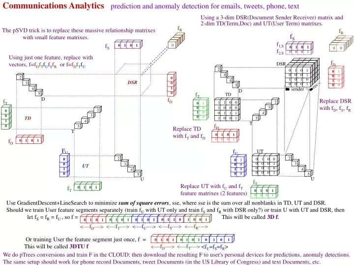
4. Comprehensive comparison of 3 alternatives DTU [em11] 2D(DT,UT,DS,DR); 3D(DTD,TDT,TUT,UUT,DDSR,SDSR,RDSR) DT 1 3 4 5 UT 3 5 4 u1 1 2 1 u2 DSR s1 s2s1 s2 1 d1 r1 d1 r2 d2 1 d2 1 1 1 1 1 1 1 1 1 1 1 1 1 1 TD1 TD2 TD3 DT1 DT2 TU1 TU2 TU3 DSR1 DSR2 U1 U2 S1 S2 1.19 1.19 1.19 1.19 1.19 1.19 1.19 1.19 1.19 1.19 1.19 1.19 1.19 1.19 DT _________ e 1 3 sse t -0.4 1.58 4 5 65.06 DTU 1.12 2.58 3.58 42.59 t2D 1.37 fT 1.19 1.19 1.19 UT 50.55 t3D 1.19 e 3 5 4 u1 1.58 3.58 2.58 1 2 1 u2 -0.4 0.58 -0.4 t1 t2 t3 fT 1.19 1.19 1.19 DSR e fS 1 1 d1 r1 -0.6 -0.6 1.19 1 1 d2 -0.6 -0.6 1.19 s1 s2 fD 1.19 1.19 e fS 1 1 d1 r2 -0.6 -0.6 1.19 1 1 d2 -0.6 -0.6 1.19 s1 s2 fD 1.19 1.19 2.57 4.26 1.88 1.38 7.33 1.389 1.38 1.389 -3.8 -3.8 9.22 -0.2 -3.8 -3.8 DT 1 3 4 5 UT 3 5 4 u1 1 2 1 u2 DSR s1 s2s1 s2 1 d1 r1 d1 r2 d2 1 d2 2.57 4.26 1.88 1.38 7.33 1.389 1.38 1.389 -3.8 -3.8 9.22 -0.2 -3.8 -3.8 TD1 TD2 TD3 DT1 DT2 TU1 TU2 TU3 DSR1 DSR2 U1 U2 S1 S2 1.55 1.78 1.45 1.38 2.21 1.384 1.38 1.384 0.64 0.64 2.48 1.14 0.64 0.64 DT _________ e 1 0 3 sse t -1.1 0.98 4 5 0 60.87 DTU 0.025 0.56 1.03 21.84 t2D 0.116 fT 1.55 1.78 1.45 UT 7.033 t3D 0.14 e 3 5 4 -0.8 0.56 0.39 1 2 1 -0.7 -0.0 -0.6 fT 1.55 1.78 1.45 DSR1 e fS 1 1 0.42 0.07 0.64 1 1 0.42 0.07 0.64 fD 1.38 2.21 DSR2 e fS 1 1 0.42 0.07 0.64 1 1 0.42 0.07 0.64 fD 1.38 2.21 -3.3 3.64 1.57 0.06 3.13 -3.00 1.34 0.203 0 -2.5 0.26 -2.2 1.50 0.41 DT 1 3 4 5 UT 3 5 4 u1 1 2 1 u2 DSR s1 s2s1 s2 1 d1 r1 d1 r2 d2 1 d2 -3.3 3.64 1.57 0.06 3.13 -3.00 1.34 0.203 0 -2.5 0.26 -2.2 1.50 0.41 TD1 TD2 TD3 DT1 DT2 TU1 TU2 TU3 DSR1 DSR2 U1 U2 S1 S2 1.29 2.06 1.57 1.38 2.45 1.159 1.48 1.399 0.64 0.45 2.50 0.97 0.75 0.67 DT _________ e 1 0 3 sse t -0.8 0.81 4 5 0 60.84 DTU -0.00 0.81 -0.0 16.44 t2D 0.1 fT 1.29 2.06 1.57 UT 3.377 t3D 0.075 e 3 5 4 -0.2 -0.1 0.06 1 2 1 -0.2 -0.0 -0.5 fT 1.29 2.06 1.57 DSR1 e fS 1 1 0.24 -0.3 0.75 1 1 0.32 -0.1 0.67 fD 1.38 2.45 DSR2 e fS 1 1 0.24 -0.3 0.75 1 1 0.32 -0.1 0.67 fD 1.38 2.45 -0.0 -0.5 0.78 0.12 1.07 -0.89 -0.3 -0.35 0 -0.6 -0.5 -1.2 1.12 -1.8 DT 1 3 4 5 UT 3 5 4 u1 1 2 1 u2 DSR s1 s2s1 s2 1 d1 r1 d1 r2 d2 1 d2 -0.0 -0.5 0.78 0.12 1.07 -0.89 -0.3 -0.35 0 -0.6 -0.5 -1.2 1.12 -1.8 TD1 TD2 TD3 DT1 DT2 TU1 TU2 TU3 DSR1 DSR2 U1 U2 S1 S2 1.29 2.04 1.59 1.39 2.48 1.132 1.47 1.389 0.64 0.43 2.48 0.94 0.79 0.62 DT _________ e 1 0 3 sse t -0.8 0.77 4 5 0 60.84 DTU 0 0.77 -0.0 15.67 t2D 0.04 fT 1.29 2.04 1.59 UT 3.314 t3D 0.03 e 3 5 4 -0.2 -0.0 0.03 1 2 1 -0.2 0.07 -0.5 fT 1.29 2.04 1.59 DSR1 e fS 1 1 0.21 -0.3 0.79 1 1 0.38 -0.0 0.62 fD 1.39 2.48 DSR2 e fS 1 1 0.21 -0.3 0.79 1 1 0.38 -0.0 0.62 fD 1.39 2.48 0.01 -0.3 0.70 -0.0 1.09 -0.77 -0.1 -0.38 0 -0.5 -0.4 -0.9 1.19 -1.7

5. Train f as follows: Train w 2D matrix, TD Train w 2D matrix UT Train over the 3D matrix, DSR fRDSR 0 1 0 0 0 fUUT 0 0 1 0 0 0 0 0 0 0 0 fDDSR fRDSR 0 0 1 1 0 0 1 1 fSDSR fSDSR 0 0 1 0 fDDSR 0 0 1 0 1 0 0 0 DSR fTTD fTTD 2 3 4 0 0 1 1 0 0 1 1 5 fDTD fDTD D T TD 2 0 2 3 0 3 1 4 4 0 5 fUUT 5 U T 0 0 1 1 0 0 1 1 fTUT fTUT UT pSVD for Communication Analytics, f = sse=nbTD(td-TDtd)2 sse=nbUT(ut-UTut)2 sse=nbDSR(dsr-DSRdsr)2 ssed=2nbTD(td-TDtd)t sseu=2nbUT(ut-UTtd)t ssed=2nbDSR(dsr-DSRdsr)sr sset=2nbTD(td-TDtd)d sset=2nbUT(ut-UTtd)u sses=2nbDSR(dsr-DSRdsr)dr sser=2nbDSR(dsr-DSRdssr)ds pSVD classification predicts blank cell values. pSVD FAUST Cluster: Use pSVD to speed up FAUST cluster by looking for gaps in TD rather than TD (i.e., using SVD predicted values rather than actual given TD values). The same goes for DT, UT, TU, DSR, SDR, RDS. E.g., on the T(d1,...,dn) table, the tth row is pSVD estimated as (ft*d1,...,ft*dn) and the dot product vot is pSVD estimated as k=1..n vk*ft*dk So we analyze gaps in this column of values taken over all rows, t. pSVD FAUST Classification: Use pSVD to speed up FAUST Classification by finding optimal cutpoints in TD rather than TD (i.e., using SVD predicted values rather than actual given TD values). Same goes for DT, UT, TU, DSR, SDR, RDS.

6. DSR 0 0 0 0 1 1 1 1 0 0 0 0 1 1 1 1 Item 0 0 0 0 0 0 0 0 0 0 0 0 1 1 1 1 1 1 1 1 0 0 0 0 1 1 1 1 0 0 0 0 0 0 0 0 0 0 0 0 0 0 0 0 1 1 1 1 rec 4  sender  3 2 1 People  Author 2 2 1 3 2 3 4 3 4 5 5 4 5 6 7  Customer 1 1 1 1 1 1 1 1 1 1 1 Enrollments 2 1 1 1 1 1 1 1 3 Doc 1 4 movie 2 Course 3 term  G 3 0 0 0 5 0 4 0 5 0 0 0 1 0 1 2 3 4 5 6 7 UT Doc 0 0 3 0 0 0 1 0 0 customer rates movie card 0 2 2 0 3 0 0 0 1 4 0 0 1 0 0 0 0 0 1 0 0 1 0 0 4 0 0 5 0 0 0 0 1 t 3 2 1 1 2 3 PI PI termterm card (share stem?) Gene 4 5 3 6 4 7 5 6 1 1 3 Gene Exp 0 0 0 0 1 0 0 0 1 0 0 0 0 0 0 0 0 customer rates movie as 5 card 0 0 0 0 0 0 0 0 0 0 0 0 0 0 0 1 0 Recalling the massive interconnection of relationships between entities, any analysis we do on this we can do after estimating each matrix using pSVD trained feature vectors for the entities. On the next slide we display the pSVD1 (one feature) replacement by a feature vector which approximates the non-blank cell values and predicts the blanks. cust item card termdoc card authordoc card genegene card (ppi) docdoc People  expPI card expgene card genegene card (ppi)

7. 1 On this slide we display the pSVD1 (one feature) replacement by a feature vector which approximates the non-blank cell values and predicts the blanks. 1 fDSR,S 1 fDSR,R Train the following feature vector thru gradient descent of sse, but that each set of matrix feature vectors be trained on only the sse over the nonblank cells of that matrix. / train these 2 on GG1 \/train these 2 on EG\/ train on GG2 \ And the same for the rest of them. Any data mining we can do with the matrixes, we can do (estimate) with the feature vectors (e.g., netflix like recommenders, prediction of blank cell values, FAUST gap based classification and clustering including anomaly detection). fUT,T fDSR,D fG5 fCI,C fG2 fUT,U fE2 Item fG4 1 1 4 fG3 3 fCI,I 2 1 fTD,T People = Author 3 4 5 6 3 4 1 2 3 4 5 6 7 2 3 4 5 2 3 2 2 3 3 4 4 5 5 =Customer=users fG1 fG1 fE,S 1 1 1 fG2 1 1 1 1 1 1 fTD,D fTD,D Doc fTT,T1 4 1 3 2 1 2 3 2 1 fE,C Course movie 3 fUM,M Gene2 1 1 fD1 fE 4 T1 G1 fD2 1 2 3 4 5 6 7 3 2 1 1 1 1 1 1 3 1 Experiment fE2 fE1 3 4 5 6 3 4 1 2 3 4 5 6 7 2 3 4 5 2 3 2 2 3 3 4 4 5 5 fTT,T2 fG5 T2 fUM,M 1 1 2 2 3 3 3 4 5 fG4 fTT,T1 G3 fG3 Doc Sender Receiver UT CI AD TD Enroll GG1 DD UserMovie ratings ExpG ExpPI TermTerm GG2

8. A n-dim vector space, RC(C1,...,Cn) is a matrix or TwoEntityRelationship (with row entity instances R1...RN and column entity instances C1...Cn.) ARC will denote the pSVD approximation of RC: d fC FC= f1C f2C fR 1 2 2 2 f1R f2R 5 5 1 1 3 5 3 3 Once f is trained and if d=unit n-vector, the SPTS, ARCfodt, is: 0 0 1 1 0 0 0 0 2 2 0 0 0 0 0 0 1 1 4 4 0 0 0 0 1 1 0 0 k=1..nfR1fCkdk = (fR1fC)odt = fR1(fCodt) 2 6 0 0 0 0 0 0 1 1 : : : : fR2(fCodt) (fR2fC)odt : k=1..nfR2fCkdk : 1 1 fR1k=1..nfCkdk = 4 1 2 4 1 0 ... ... ... 3 5 0 k=1..nfRNfCkdk fR2k=1..nfCkdk : (fRNfC)odt fRN(fCodt) fRNk=1..nfCkdk Once F is trained and if d=unit n-vector, the SPTS, ARCodt, is: k=1..n(f1R1f1Ck+..+fKR1fKCk)dk = (FR1oFC)odt = FR1o(FCodt) k=1..n(f1R2f1Ck+..+fKR2fKCk)dk : FR2o(FCodt) : (FR2oFC)odt : k=1..n(f1RNf1Ck+..+fKRNfKCk)dk FRNo(FCodt) (FRNoFC)odt A N+n vector, f=(fR, fC) defines prediction, pi,j=fRifCj, error, ei,j=pi,j-RCi,j then ARCf,i,j≡fRifCj and ARCf,row_i= fRifC= fRi(fC1...fCn)= (fRifC1...fRifCn). Use sse gradient descent to train f. RC C1 C2 ... Cn R1 R2 . . . RN 0 1 0 0 0 0 0 1 0 0 1 0 0 0 0 1 Compute fCodt=k=1..nfCkdk form constant SPTS with it, and multiply that SPTS by SPTS, fR. Any datamining that can be done on RC can be done using this pSVD approximation of RC, ARC e.g., FAUST Oblique (because ARCodt should show us the large gaps quite faithfully). Given any K(N+n) feature matrix, F=[FR FC], FRi=(f1Ri...fKRi), FCj=(f1Cj...fKCj) pi,j=fRiofCj=k=1..KfkRifkCj Keeping in mind that we have decided (tentatively) to approach all matrixes as rotatable tables, this then is a universal method of approximation. The big question is, how good is the approximation for data mining? It is known to be good for Netflix type recommender matrixes but what about others?

9. e 1 2 3 4 5 6 7 8 9 a b 1 2 3 4 5 6 7 8 9 a b c d e f -.2 .07 .21 -.1 .94 0.000 0.262 0.238 0.000 0.102 0.081 0.000 0.000 0.000 fR fC Of course if we take the previous data (all nonblarnks=1. and we only count errors in those nonblarnks, then f pure1 is error=0. But of course, if it is an image (fax-type image of 0/1) then there are no blanks (and zero positions must be assessed error too). So we change the data. t sse .13 .2815 1 2 3 4 5 6 7 8 9 a b 1 1 2 5 3 2 3 4 5 6 3 7 2 8 9 4 3 10 1 11 3 4 12 13 1 14 5 15 2