Download
1 / 42
420 likes | 484 Views
A parametric and process-oriented view of the carbon system. The challenge: explain the controls over the system’s response. Carbon emissions and uptakes since 1800 (Gt C). Expanding the model:. A model for (F ba -F ab ) F ab = G(D i , p i , S i ) = photosynthesis

E N D
The challenge: explain the controls over the system’s response
Expanding the model: A model for (Fba-Fab) Fab = G(Di, pi, S i) = photosynthesis Fba = G(Di, pi, S i) = respiration and fire
A Hierarchical view of the carbon system Causation goes in this direction Drivers (weather, nutrients, fires) Fluxes Concentrations Inverse models do something is this direction
A-R: A key feature of the system What we measure: Net Ecosystem Exchange (the flux of CO2 across an imaginary plane above the canopy) But: NEE cannot be directly parameterized NEE = Photosynthesis - Respiration The model (or observation equation) must “transform” the observation (NEE) into physically modeling components. This is neglecting complex but different processes such as fire and forest harvest.
Ecosystem Model Structure Photosynthesis (Phenology,Soil Moisture, Tair, VPD, PAR) Plant Respiration (Plant C, Tair) Plant Carbon Precip. Transpiration Litterfall (Plant C, Phenology) Soil Respiration (Soil C, Soil Moisture, Tsoil) Soil Moisture Soil Carbon Drainage
Some key model equations NEE = Ra +Rh - GPP GPPmax = AamaxAd+Rleaf GPPpot = GPPmaxDtempDvpdDlight Rh = CsKhQ10sTsoil/10(W/Wc) GPP = canopy photosynthesis, R denotes respiration, Amax = max leaf-level carbon assimilation, Ds are scalars for environmental factors, Ad, a scaling factor over time, Cs = substrate, K, rate constant, Q10 the temperature scalar and W, water scalars.
Estimation (zj - H(Fapj,Fpaj))tR-j1 (zj - H(Fapj,Fpaj))/2 + (pj - Pj)tR-j1 (pj - Pj) /2 The rubber bands are the prior estimates of parameters
Assimilation of fluxes provides consistency between prior knowledge and observed carbon exchange
Control variables • Temperature • Soil moisture • Nutrient availability • Fire regime • Light interception • Land management • Atmospheric CO2 • etc
Concentrations have less information about processes and parameters than do fluxes Why? They are “one step more removed” (by transport) That step includes “invertible” (advective) processes and irreversible (diffusive) processes There is information loss along the chain of causation
Get closer to the answer: measure fluxes Tower-based measurements
More gadgets My little flux tower….
More gadgets CO2, H2O T, u,v,w w
Time-scale character of carbon modeling Variability is at a maximum on the strongly forced time scales They have an annual sum of ~0 Modeling the carbon storage time scales (years) is the goal Diurnal Seasonal
Analysis of controls Warm springs accelerate growth but also evaporation. Despite the overall positive response shown earlier, the annual relationship of flux to temperature is negative
Self-consistent parameter sets Fit to the diurnal cycle (~12 hour time steps) Fit to daily data: 24 hour time steps
Assimilating water and carbon Just water Carbon only or carbon plus water
Adding water doesn’t help carbon, but it helps water Carbon only Carbon and water
KH (g g-1 y-1) CS,0 (g m-2) Self-consistent parameter sets Range from prior knowledge Validate-tune Second parameter dictated First parameter
Analysis of controls The emergent Relationship of temperature and carbon uptake. Note the multiple Regimes. The lower lines are the water-limited response Realized T response wet Realized T response, dry
What does this type of local study contribute to global modeling? We can use this to understand the information in different types of observation
Carbon from space OCO uses reflected sunlight to make measurements during the day
Day and Night Remember, we’ve shown a huge loss of process information without diurnal information
Future active CO2 experiments make day and night observations LIDAR
Process priors for global models Tower-based estimates of parameters can be used as priors to invert global concentration data to estimate parameters controlling fluxes instead of fluxes (Knorr, Wofsy, Rayner)
The global scale is very distant from processes Distributed local measurements and innovative measurement approaches can bridge the gap
Carbon dataassimilation Carbon data assimilation and parametric estimation are fast-moving fields
A few references • Vukicevic, T., B.H. Braswell and D.S. Schimel. 2001. A diagnostic study of temperature controls on global terrestrial carbon exchange. Tellus (B) 53:150-170. (variational) • Braswell, B.H., W.J. Sacks, E. Linder and D.S. Schimel. 2004. Estimating ecosystem process parameters by assimilation of eddy flux observations of NEE. Global Change Biol. 11:335-355 (MCMC) • Williams, M. Schwarz, B.E. Law, J. Irvine, and M.R. Kurpius. 2005. An improved analysis of forest carbon dynamics using data assimilation. Glov=bal Change Biol. 11:85-105 (EKF) • Wang, Y-P. and D Barrett. 2003. stimating regional terrestrial carbon fluxes for the Australian continent using a multiple-constraint approach. I. Using remotely sensed data and ecological observations of net primary production. Tellus (B) 55:270-289 (Synthesis inversion)