Download
1 / 75
760 likes | 778 Views
Consumer Choice: Indifference Theory. The basic assumption here is that consumers are motivated to make themselves as well off as they can, or as economists like to put it: to maximize their satisfaction, or utility.

E N D
The basic assumption here is that consumers are motivated to make themselves as well off as they can, or as economists like to put it: to maximize their satisfaction, or utility.
All units of the same product are identical but the satisfaction that a consumer gets from each unit of a product is not the same. This suggests that the satisfaction that people get from consuming a unit of any product varies according to how many units of this product they have already.
Economists and philosophers thinking about consumer choice and satisfaction in the nineteenth century developed the concept of utility and were hence sometimes called utilitarians. But the big breakthrough for economics came in the 1870s with what is known as the marginal revolution, which gave birth to neoclassical economics.
Decision Making Process of the consumer: • Preference Set: It is a comprehensive set of all preferences of the consumer. • Opportunity set: It consists of combinations of the two goods that the consumer can buy given that there is a limited income that one can spend on these goods.
Preference set under these assumptions: • Assumption of completeness: When a consumer is confronted with any of the two goods or two basket of goods, she is able to express that she prefers one or the other or whether she is indifferent. • Assumption of Transitivity: If a consumer prefers A to B and prefers B to C, then she will prefer A to C
3. Assumption of Non-Satiation: A rational consumer prefers more of a good to less of the good.
Marginal and total utility The satisfaction a consumer receives from consuming that product is called utility. Total utility refers to the total satisfaction derived from all the units of that product consumed. Marginal utility refers to the change in satisfaction resulting from consuming one unit more or one unit less of that product.
Total and Marginal Utility Schedules Number of films attended per month Total utility Marginal utility 0 0.00 1 15.00 15.00 2 25.00 10.00 3 31.00 6.00 4 35.00 4.00 5 37.50 2.50 6 39.00 1.5 7 40.25 1.25 8 41.30 1.05 9 42.20 0.90 10 43.00 0.80
As consumption increases, total utility rises but marginal utility falls. The marginal utilities are the changes in utility when consumption is altered by one unit. For example, the marginal utility of 10m, shown in the entry in the last column, arises because with attendances at the second film total utility increase from 15 to 25 a difference of 10. The data in this table are plotted in the following figure. Total and Marginal Utility Schedules
Total and Marginal Utility Curves 50 20 Utility [£] 40 Utility [£] 15 30 20 10 10 5 0 2 4 6 8 10 0 2 4 6 8 10 Quantity of films [attendance per month] [i]. Increasing total utility [ii]. Diminishing marginal utility
Diminishing marginal utility A basic assumption of utility theory, which is sometimes called the law of diminishing marginal utility, is as follows: The marginal utility generated by additional units of any product diminishes as an individual consumes more of it, holding constant the consumption of all other products.
Maximizing utility We can now ask: what does diminishing marginal utility imply for the way a consumer who has a given income will allocate spending in order to maximize total utility? How should a consumer allocate his or her income in order to get the greatest possible satisfaction, or total utility, from that spending?
Optimization – Cardinal Approach • Optimization Rule 1: When unlimited quantity of a good is available for no cost and the individual has to consume successive units of the commodity at the same point in time, a rational consumer willmaximise total utility by consuming till the point where marginal utility is zero. MUx = 0
Total and Marginal Utilities from Ice Cream Consumption for Individual
Optimization Rule 2: When only one good is consumed and is available for a price: Consume till MUx = Pricex
Optimization Rule 3: Law of Equi Marginal Utility or Law of Substitution : The law states that the consumer will spend his income on different goods in such a way that marginal utility of each good is proportional to it’s price ie. when more than one good is consumed and the goods’ prices are different: Consume till MUx/Px = MUy/Py = MUz/Pz
If one product had a higher marginal utility than the others, then expenditure should be reallocated so as to buy more of this product, and less of all others that have lower marginal utilities. By buying more, its marginal utility would fall. This continues until the consumer's utility equates to his/her expenditure and utility is maximized.
How does this work if products have different prices? Again, the same principles apply but now the best a consumer can do is to rearrange spending until the last unit of satisfaction per pound spent on each product is the same.
The rule is to carry on allocating additional rupees to the commodity until the marginal utility derived from the last additional rupee is the same irrespective of the commodity that it is spent on, and the income is exhausted.
Conditions for maximising utility The conditions for maximizing utility can be stated more generally. Denote the marginal utility of the last unit of product X by MUX and its price by pX. Let MUY and pY refer, respectively, to the marginal utility of a second product, Y, and its price. The marginal utility per pound spent on X will be MUX/pX.
The condition required for any consumer to maximize utility is that the following relationship should hold, for all pairs of products:
This is the fundamental equation of utility theory. Each consumer demands each good up to the point at which the marginal utility per pound spent on it is the same as the marginal utility of a pound spent on each other good. When this condition is met, the consumer cannot shift a pound of spending from one product to another and increase total utility.
Consumers choose quantities not prices If we rearrange the terms in previous equation we can gain additional insight into consumer behaviour:
The right-hand side of this equation states the relative price of the two goods. It is determined by the market and is beyond the control of individual consumers, who react to these market prices but are powerless to change them.
The left-hand side of the equation states the relative contribution of the two goods to add to satisfaction if a little more or a little less of either of them were consumed, a choice that is available.
When they enter the market, all consumers face the same set of market prices. When they are fully adjusted to these prices, each one of them will have identical ratios of their marginal utilities for each pair of goods.
A rich consumer may consume more of each product than a poor consumer and get more total utility from them. However, the rich and the poor consumer (and every other consumer who is maximizing utility) will adjust their relative purchases of each product so that the relative marginal utilities are the same for all.
Consumers with different tastes will, however, derive different marginal utilities from their consumption of the various commodities. So they will consume differing relative quantities of products
Consumers Surplus A consumer surplus occurs when the consumer is willing to pay more for a given product than the current market price. Consumers always like to feel like they are getting a good deal on the goods and services they buy and consumer surplus is simply an economic measure of this satisfaction. For example, assume a consumer goes out shopping for a CD player and he or she is willing to spend $250. When this individual finds that the player is on sale for $150, economists would say that this person has a consumer surplus of $100.
Consumer’s Surplus for an Individual 3.00 2.00 Price of milk [£ per glass] 1.00 Market price 0.30 1 2 3 4 5 6 7 8 9 10 Glasses of milk consumed per week
Consumer’s surplus is the sum of the extra valuations placed on each unit above the market price paid for each. This figure is based on the data in the table. Ms.Green pays the red area for the 8 glasses of milk she consumes per week when the market price is £0.30 a glass. The total value she places on these 8 glasses of milk is the entire shaded area (red and green). Hence her consumer’s surplus is the green area. Consumer’s Surplus for an Individual
The Utility Theory of Demand Marginal utility theory distinguishes between the total utility that each consumer gets from the consumption of all units of some product and the marginal utility each consumer obtains from the consumption of one more unit of the product. The basic assumption in utility theory is that the utility the consumer derives from the consumption of successive units of a product diminishes as the consumption of that product increases. Each consumer reaches a utility-maximizing equilibrium when the utility he or she derives from the last £1 spent on each product is equal.
Another way of putting this is that the marginal utilities derived from the last unit of each product consumed will be proportional to their prices. Demand curves have negative slopes because when the price of product X falls, each consumer restores equilibrium by increasing his or her purchases of X. The increase must be enough to lower the marginal utility of X until its ratio to the new lower price of X is the same as it was before the price fell. This restores the equality of the ratio to what it is for all other products. MARGINAL UTILITY
Consumers’ Surplus Consumers’ surplus is the difference between [1] the value consumers place on their total consumption of some product and [2] the actual amount paid for it. The first value is measured by the maximum they would pay for the amount consumed rather than go without it completely. The second is measured by market price times quantity. MARGINAL UTILITY
It is important to distinguish between total and marginal values because choices concerning a bit more and a bit less can not be predicted from knowledge of total values. The paradox of value involves confusion between total and marginal values. Elasticity of demand is related to the marginal value that consumers place on having a bit more or a bit less of some product; it bears no necessary relationship to the total value that consumers place on all of the units consumed of that product. MARGINAL UTILITY
Indifference Curve – Ordinal Approach An indifference curve shows combinations of products that yield the same satisfaction to the consumer. The amount of Y that the individual would be willing to give up for X is called the marginal rate of substitution i.e. slope of the indifference curve.
Bundles Conferring Equal Satisfaction Bundle Clothing Food A B C D E F 30 18 13 10 8 7 5 10 15 20 25 30
Bundles Conferring Equal Satisfaction 35 a 30 25 g Quantity of clothing per week 20 b 15 c d 10 e f h T 5 5 10 15 20 25 30 35 Quantity of food Ranking commodity bundles : g is preferred to b & c; b& c is preferred to h
None of the bundles in the table are obviously superior to any of the others in the sense of having more of both commodities. Since each of the bundles shown in the table give the consumer equal satisfaction, he is indifferent between them. Bundles Conferring Equal Satisfaction
Indifference Curves • Properties of Indifference curves: - Slope downward: Whenever quantity of one good increases, quantity of the other good decreases. - Convex to the origin and are based on the principle of diminishing marginal rate of substitution. Absolute value of MRS has to decrease as the consumer moves away from the origin on the X - axis - Non intersecting : If two indifference curves crossed, it would mean that one of them refers to a higher level of satisfaction than the other at one side of the intersection and to a lower level of satisfaction at the other side of the intersection.
An Indifference Map Quantity of food per week I5 I4 I3 I2 I1 Quantity of food per week 0
A set of indifference curves is called an indifference map. The further the curve from the origin, the higher the level of satisfaction it represents. Moving along the arrow is moving to ever-higher utility levels. An Indifference Map
Shapes of Indifference Curves Perfect Substitutes Perfect Complements Left hand gloves I2 I2 I1 I1 0 0 [i]. Packs of green pins [ii]. Right hand gloves
Perfect substitutes are having a constant rate of substitution at all levels of consumption. Complements are consumed in fixed proportions.
Shapes of Indifference Curves A good that confers a negative utility after some level of consumption An absolute necessity I2 I1 All other goods All other goods A good that confers a negative utility after some level of consumption I2 I1 0 w 0 f0 0 [iv]. Water [v]. Food The marginal rate of substitution for an absolute necessity approaches infinity as consumption falls towards the amount that is absolutely necessary.
Opportunity Set • Defined by Budget Constraint. 6x + 3y = 60 Given Px = 6 and Py = 3 • If the consumer spends all his income only on X, he can purchase 10 units of X, while if he spends all his income on Y, he can purchase 20 units of Y. Combination of income spent on X and Y gives the Budget Line • A change in income, with no change in prices, will lead to a parallel shift in the budget line. • Slope of the budget line changes only when the relative prices change other things remaining the same -Px/Py is the Slope
Consumer Equilibrium • The goal of the consumer is to buy the affordable quantities of goods that make the consumer as well off as possible. • The consumer’s preference map describe the way a consumer values different combinations of goods. • The consumer’s budget and the prices of the goods limit the consumer’s choices.